# Extra packages this lesson
pacman::p_load(
  nanoparquet, # loads parquet files faster
  tidyquant    # tq_get
)Introduction to Non-stationary Models and Differencing
Chapter 7: Lesson 1
Learning Outcomes
Explain the concept of non-stationarity in time series
- Define non-stationarity and its implications for time series analysis
- Identify non-stationary behavior in time series plots
Apply differencing to remove non-stationarity
- Explain the concept of differencing and its role in removing non-stationarity
- Use differencing to transform non-stationary time series into stationary ones
- Interpret the results of differencing on time series plots and ACF/PACF
Identify integrated models and ARIMA notation
- Define integrated models and their relationship to differencing
- Understand the ARIMA notation and its components (p, d, q)
- Recognize the role of the ‘d’ parameter in ARIMA models
Preparation
- Read Sections 7.1-7.2
- Read Prof. Frenzel’s Blog Post
Learning Journal Exchange (10 min)
Review another student’s journal
What would you add to your learning journal after reading another student’s?
What would you recommend the other student add to their learning journal?
Sign the Learning Journal review sheet for your peer
Packages
pacman::p_load(
  tidyverse,  # ggplot, mutate(), cleaning...
  tsibble,    # as_tsibble()
  fable,      # model(...), forecast(), tidy(), glance()...
  feasts,     # ACF(), PACF()
  ggtime,     # autoplot() for tsibbles
  patchwork,  # + and / for ggplots
  rio         # import()
)
Class Activity: Non-seasonal ARIMA Models (15 min)
Effect of Differencing
In Chapter 4 Lesson 2, we found that if we compute the first difference of the price of McDonald’s stock from July 2020 through December 2023, the differences can be modeled as white noise. Sometimes differencing can remove trends.
Consider the case of a random walk and a linear trend with white noise errors
Random Walk
Linear Trend with White Noise Errors
Fitting an ARIMA Model when the Difference Model has a Non-Zero Mean
(See the last sentence in the first paragraph on page 138.)
Differencing a Time Series or the Logarithm of a Time Series
If the difference of a time series demonstrates an increasing trend, taking the logarithm before differencing can eliminate the increasing variation in the differences. As an example, consider the Australian electricity production series given in the book.
Show the code
cbe <- read_table("https://byuistats.github.io/timeseries/data/cbe.dat") |>
  select(elec) |>
  mutate(
    date = seq(
      ymd("1958-01-01"),
      by = "1 months",
      length.out = n()),
      year_month = tsibble::yearmonth(date)) |>
  as_tsibble(index = year_month)

cbe |>
  mutate(
    `Diff series` = elec - lag(elec),
    `Diff log-series` = log(elec) - lag(log(elec))) |>
  pivot_longer(
    cols = all_of(c("elec", "Diff series", "Diff log-series"))) |>
  mutate(name = factor(name, levels =c("elec","Diff series", "Diff log-series"))) |>
  ggplot(aes(x = date, y = value)) +
  geom_line() +
  facet_wrap(~name, ncol = 1, scales = "free", strip.position = "left") +
  labs(x = "Time", y = "") +
  scale_x_date(breaks = "5 years", date_labels = "%Y") +
  theme_bw()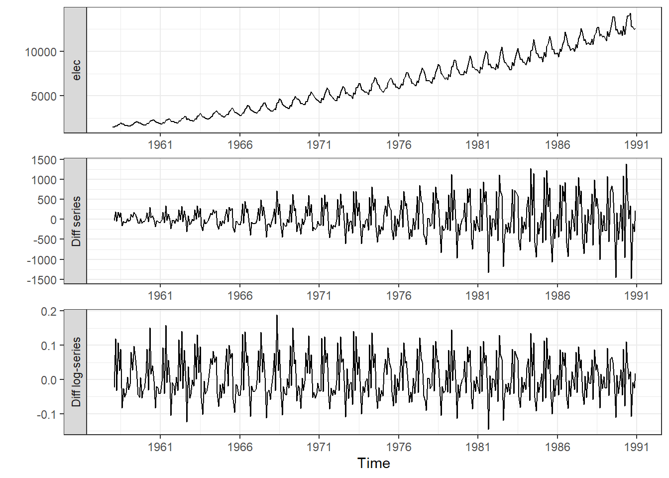
Integrated Time Series of Order d
Recall that \(\nabla^d \equiv \left( 1 - \mathbf{B} \right)^d\). So, either of the following can be used to indicate an integrated time series of order \(d\):
\[\begin{align*} \nabla^d x_t &= w_t \\ ~\\ \left( 1 - \mathbf{B} \right)^d x_t &= w_t \end{align*}\]
Special Case: \(I(1)\)
Second-Order Differencing and Lagged Differences
A linear trend can be removed by first-order differencing. A curved trend can sometimes be eliminated by second order differencing.
In some cases, a lagged difference is more appropriate. For example, if you have monthly data and need to remove additive seasonal effects, you may want to take a difference with a lag of 12. This subtracts sequential January observations from each other. This models the year-over-year growth.
Notice that taking a lag 12 difference
\[ \left( 1 - \mathbf{B}^{12} \right) x_t = x_t - x_{t-12} \]
is very different from taking the twelfth differences
\[\begin{align*} \nabla^{12} x_t &= \left( 1 - \mathbf{B} \right)^{12} x_t \\ &= x_t - 12 x_{t-1} + 66 x_{t-2} - 220 x_{t-3} + 495 x_{t-4} - 792 x_{t-5} + 924 x_{t-6} \\ & ~~~~~~~~~~~~~~~~~~~ - 792 x_{t-7} + 495 x_{t-8} - 220 x_{t-9} + 66 x_{t-10} - 12 x_{t-11} + x_{t-12} \end{align*}\]
ARIMA Process
ARIMA
Suppose we let \(y_t = \left( 1 - \mathbf{B} \right)^d x_t\). The series \(\{y_t\}\) follows an \(ARMA(p,q)\) process if \(\theta_p \left(\mathbf{B} \right) y_t = \phi_q \left(\mathbf{B} \right)w_t\).
Substituting, we find that \(\{x_t\}\) follows an \(ARIMA(p,d,q)\) process if
\[ \theta_p \left(\mathbf{B} \right) \left( 1 - \mathbf{B} \right)^d x_t = \phi_q \left(\mathbf{B} \right) w_t \]
where \(\theta_p \left(\mathbf{B} \right)\) and \(\phi_q \left(\mathbf{B} \right)\) are polynomials of orders \(p\) and \(q\), respectively.
Special Case: \(IMA(d,q)\) Process
Special Case: \(ARI(p,d)\) Process
Simulating an ARIMA Process
We can simulate data from the ARIMA process
\[ x_t = 0.5 x_{t-1} + x_{t-1} - 0.5 x_{t-2} + w_t + 0.3 w_{t-1} \]
using the following R code.
set.seed(1)
n <- 10000
x <- rnorm(n)
w <- rnorm(n)
for (i in 3:n) {
  x[i] <- 0.5 * x[i - 1] + x[i - 1] - 0.5 * x[i - 2] + w[i] + 0.3 * w[i - 1]
}
arima(x, order = c(1, 1, 1))
Call:
arima(x = x, order = c(1, 1, 1))

Coefficients:
         ar1     ma1
      0.4811  0.3170
s.e.  0.0125  0.0134

sigma^2 estimated as 0.9814:  log likelihood = -14094.25,  aic = 28194.49
This is an ARIMA(1,1,1) process with parameters \(\alpha = 0.5\) and \(\beta = 0.3\).
Class Activity: Fitting an ARIMA Process - Exchange Rates (10 min)
The data file exchange_rates.parquet gives the exchange rates for foreign currencies. The daily-observed values in the time series are the amount in the foreign currency equivalent to one U. S. dollar. We will consider the exchange rates to convert one dollar into Euros.
Show the code
exchange_ts <- rio::import("data/exchange_rates.parquet") |>
  filter(currency == "USD.EUR") |>
  as_tsibble(index = date) |>
  na.omit()

exchange_ts |>
display_partial_table(6,3)| date | currency | rate |
|---|---|---|
| 2023-08-24 | USD.EUR | 0.922 |
| 2023-08-25 | USD.EUR | 0.926 |
| 2023-08-26 | USD.EUR | 0.926 |
| 2023-08-27 | USD.EUR | 0.926 |
| 2023-08-28 | USD.EUR | 0.925 |
| 2023-08-29 | USD.EUR | 0.923 |
| ⋮ | ⋮ | ⋮ |
| 2026-05-03 | USD.EUR | 0.853 |
| 2026-05-04 | USD.EUR | 0.854 |
| 2026-05-05 | USD.EUR | 0.855 |
Show the code
exchange_ts |>
  autoplot(.vars = rate) + labs(title = exchange_ts$currency[1])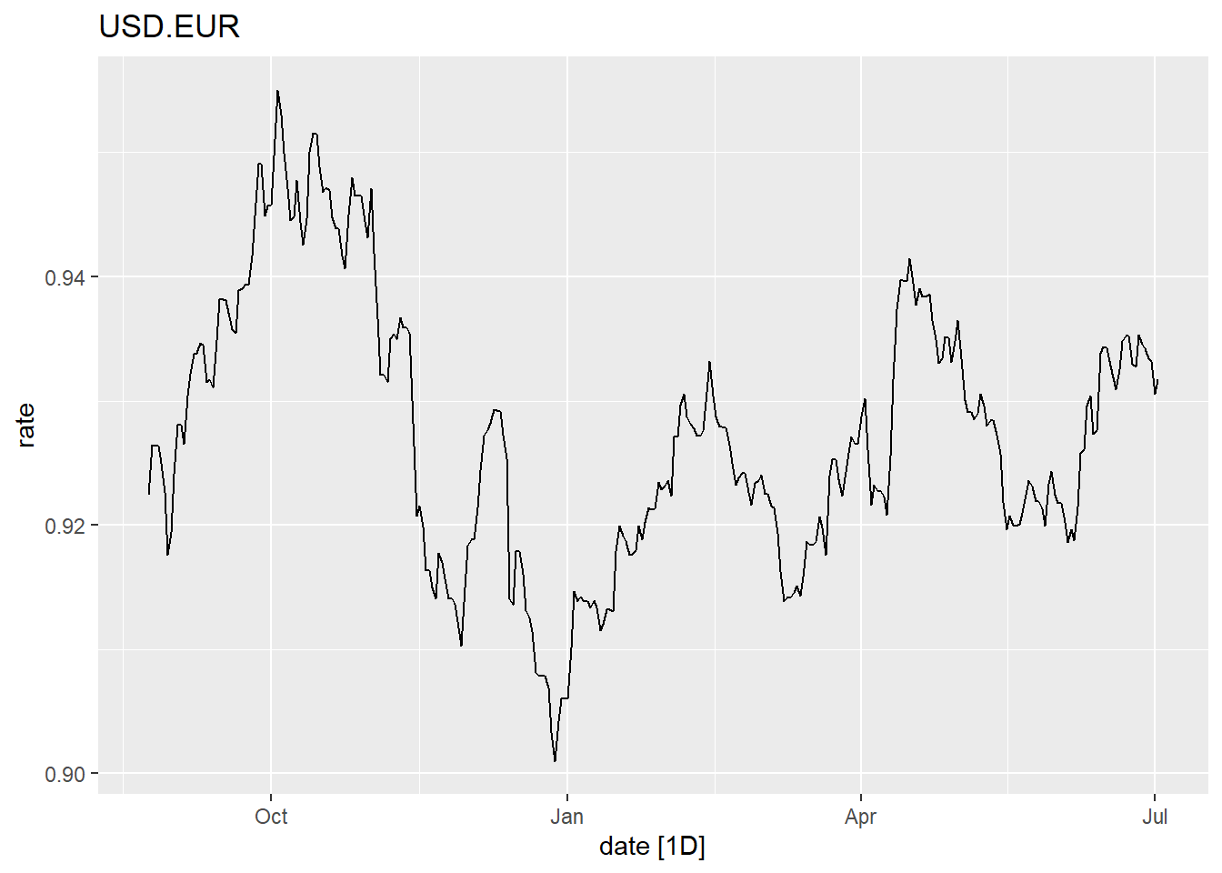
Show the code
exchange_ts <- exchange_ts |> tsibble::fill_gaps()

acf_plot <- exchange_ts  |> select(rate) |> ACF() |> autoplot(var = .resid)

pacf_plot <- exchange_ts   |> select(rate) |> PACF() |> autoplot(var = .resid)

acf_plot | pacf_plot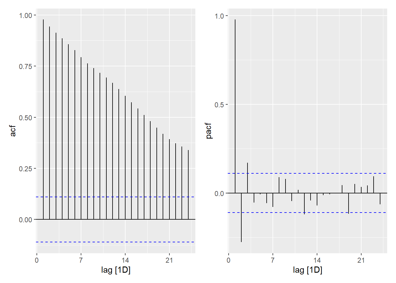
# Fit the ARIMA Model

exchange_model <- exchange_ts |>
  model(
    auto = ARIMA(rate ~ 1 + pdq(0:2,0:1,0:2) + PDQ(0, 0, 0)),

    a000 = ARIMA(rate ~ 1 + pdq(0,0,0) + PDQ(0, 0, 0)),
    a001 = ARIMA(rate ~ 1 + pdq(0,0,1) + PDQ(0, 0, 0)),
    a002 = ARIMA(rate ~ 1 + pdq(0,0,2) + PDQ(0, 0, 0)),
    a100 = ARIMA(rate ~ 1 + pdq(1,0,0) + PDQ(0, 0, 0)),
    a101 = ARIMA(rate ~ 1 + pdq(1,0,1) + PDQ(0, 0, 0)),
    a102 = ARIMA(rate ~ 1 + pdq(1,0,2) + PDQ(0, 0, 0)),
    a200 = ARIMA(rate ~ 1 + pdq(2,0,0) + PDQ(0, 0, 0)),
    a201 = ARIMA(rate ~ 1 + pdq(2,0,1) + PDQ(0, 0, 0)),
    a202 = ARIMA(rate ~ 1 + pdq(2,0,2) + PDQ(0, 0, 0)),

    a011 = ARIMA(rate ~ 1 + pdq(0,1,1) + PDQ(0, 0, 0)),
    a012 = ARIMA(rate ~ 1 + pdq(0,1,2) + PDQ(0, 0, 0)),
    a110 = ARIMA(rate ~ 1 + pdq(1,1,0) + PDQ(0, 0, 0)),
    a111 = ARIMA(rate ~ 1 + pdq(1,1,1) + PDQ(0, 0, 0)),
    a112 = ARIMA(rate ~ 1 + pdq(1,1,2) + PDQ(0, 0, 0)),
    a210 = ARIMA(rate ~ 1 + pdq(2,1,0) + PDQ(0, 0, 0)),
    a211 = ARIMA(rate ~ 1 + pdq(2,1,1) + PDQ(0, 0, 0)),
    a212 = ARIMA(rate ~ 1 + pdq(2,1,2) + PDQ(0, 0, 0))
    )
Here is one way to determine which model is selected by the “auto” process.
Show the code
exchange_model |>
  select(auto)
# A mable: 1 x 1
auto
<model>
1 <ARIMA(1,1,2) w/ drift>We now examine all the fitted models to determine the value of the residual mean squared error (sigma2), log-likelihood, AIC, AICc, and BIC. For the log-likelihood, larger values are preferable. For all other measures, smaller values are preferred.
Show the code
exchange_model |>
glance()| Model | sigma2 | log_lik | AIC | AICc | BIC |
|---|---|---|---|---|---|
| auto | 0 | 3876.9 | -7743.9 | -7743.8 | -7719.4 |
| a000 | 0 | 1627.2 | -3250.4 | -3250.4 | -3240.6 |
| a001 | 0 | 2181.8 | -4357.5 | -4357.5 | -4342.8 |
| a002 | 0 | 2632.3 | -5256.6 | -5256.6 | -5237 |
| a100 | 0 | 3836.4 | -7666.8 | -7666.8 | -7652.2 |
| a101 | **0** | 3879.6 | -7751.2 | -7751.1 | -7731.6 |
| a102 | 0 | 3879.6 | -7749.3 | -7749.2 | -7724.8 |
| a200 | 0 | 3875.1 | -7742.3 | -7742.2 | -7722.7 |
| a201 | 0 | 3879.7 | -7749.4 | -7749.4 | -7724.9 |
| a202 | 0 | **3881.7** | **-7751.4** | **-7751.3** | -7722 |
| a011 | 0 | 3876.9 | -7747.7 | -7747.7 | **-7733.1** |
| a012 | 0 | 3877 | -7746 | -7746 | -7726.4 |
| a110 | 0 | 3872.3 | -7738.5 | -7738.5 | -7723.8 |
| a111 | 0 | 3877.1 | -7746.1 | -7746.1 | -7726.5 |
| a112 | 0 | 3876.9 | -7743.9 | -7743.8 | -7719.4 |
| a210 | 0 | 3875.8 | -7743.7 | -7743.6 | -7724.1 |
| a211 | 0 | 3877.8 | -7745.6 | -7745.5 | -7721.1 |
| a212 | 0 | 3877.8 | -7743.6 | -7743.5 | -7714.2 |
Suppose we choose to apply the “auto” model, which is \(ARIMA(1,1,1)\). The model parameters are summarized here:
Show the code
exchange_model |>
  select(auto) |>
coefficients()| .model | term | estimate | std.error | statistic | p.value |
|---|---|---|---|---|---|
| auto | ar1 | 0.1535757 | NaN | NaN | NaN |
| auto | ma1 | 0.1741877 | NaN | NaN | NaN |
| auto | ma2 | -0.0650455 | NaN | NaN | NaN |
| auto | constant | -0.0000557 | 9.31e-05 | -0.5985738 | 0.5496168 |
The following plots give the acf and pacf of the residuals from this model.
Show the code
model_resid <- exchange_model |>
  select(auto) |>
  residuals()

acf_plot <- model_resid |> ACF() |> autoplot(var = .resid)

pacf_plot <- model_resid |> PACF() |> autoplot(var = .resid)

acf_plot | pacf_plot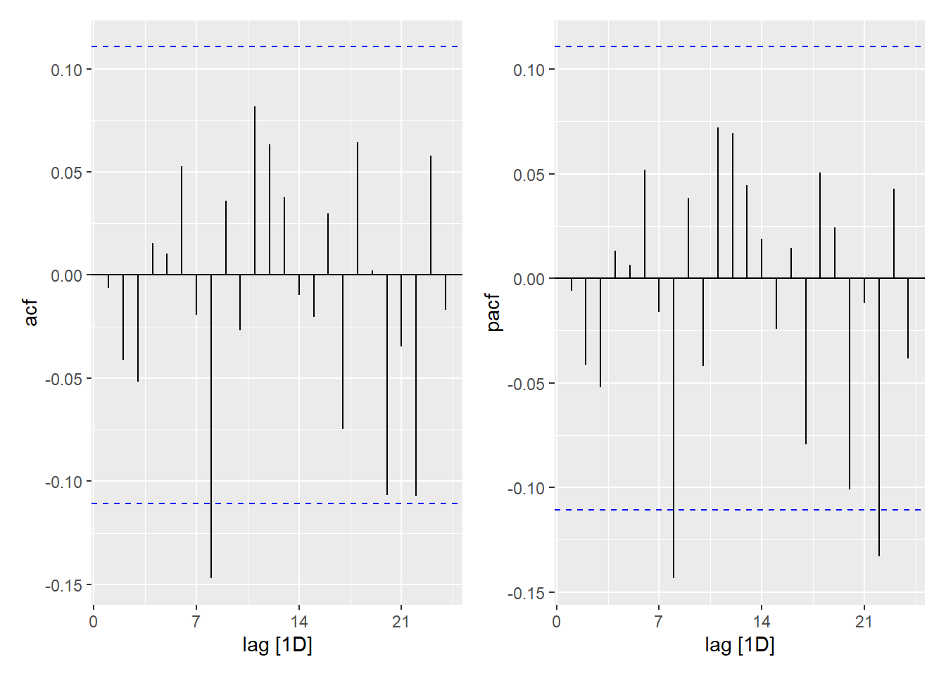
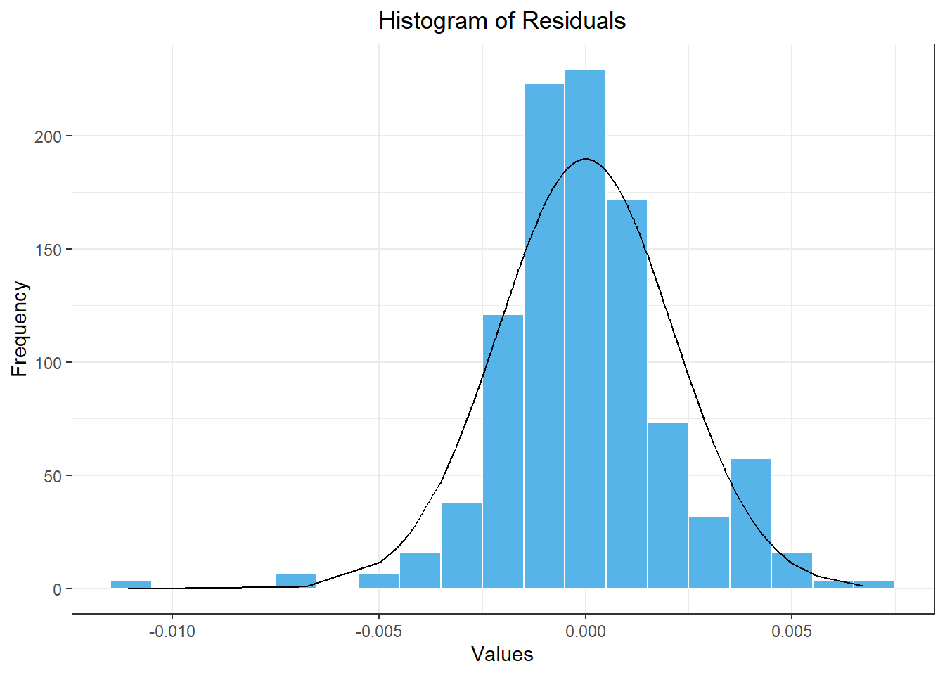
Here is a histogram of the residuals from our model.
Show the code
model_resid |>
  mutate(density = dnorm(.resid, mean(model_resid$.resid), sd(model_resid$.resid))) |>
  ggplot(aes(x = .resid)) +
    geom_histogram(aes(y = after_stat(density)),
        color = "white", fill = "#56B4E9", binwidth = 0.001) +
    geom_line(aes(x = .resid, y = density)) +
    theme_bw() +
    labs(
      x = "Values",
      y = "Frequency",
      title = "Histogram of Residuals"
    ) +
    theme(
      plot.title = element_text(hjust = 0.5)
    )
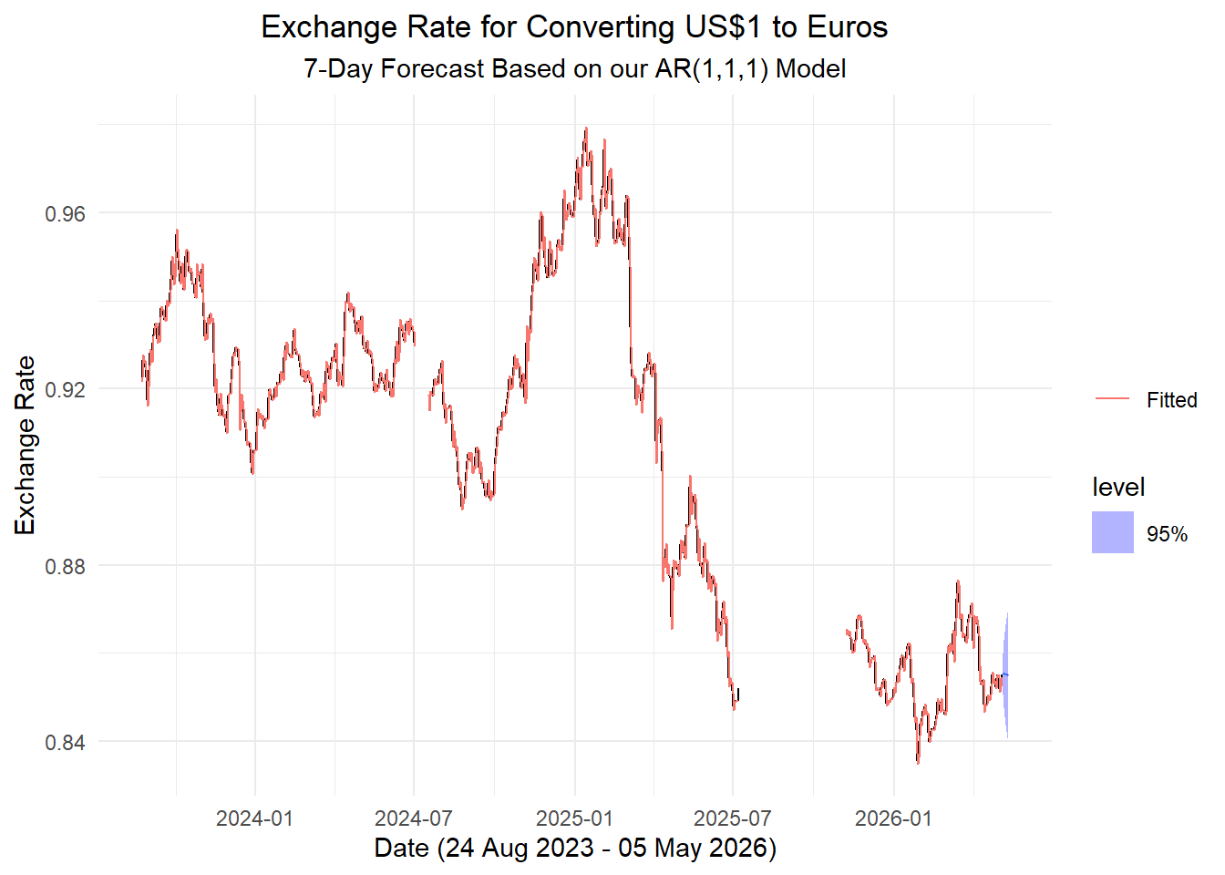
Here is a forecast for the next 7 days based on our model.
final_model <- exchange_model |>
  select(auto)

temps_forecast <- final_model |>
  select(auto) |>
  forecast(h = "7 days")

temps_forecast |>
  autoplot(exchange_ts, level = 95) +
  geom_line(aes(y = .fitted, color = "Fitted"),
    data = augment(final_model)) +
  scale_color_discrete(name = "") +
  labs(
    x = paste0(
                "Date (",
                format(ymd(min(exchange_ts$date)), "%d %b %Y"),
                  " - ",
                format(ymd(max(exchange_ts$date)), "%d %b %Y"),
                ")"
              ),
    y = "Exchange Rate",
    title = "Exchange Rate for Converting US$1 to Euros",
    subtitle = "7-Day Forecast Based on our AR(1,1,1) Model"
  ) +
  theme_minimal() +
  theme(
    plot.title = element_text(hjust = 0.5),
    plot.subtitle = element_text(hjust = 0.5)
  )
Small-Group Activity: Fitting an ARIMA Process - Microsoft Stock Prices (20 min)
A time series given the daily closing price for Microsoft (MSFT) stock is given below. To handle the gaps in the data, we define a new variable, t, which gives the observation number.
Show the code
# Set symbol and date range
symbol <- "MSFT"                # Abercrombie & Fitch stock trading symbol
date_start <- "2020-01-01"
date_end <- "2024-03-28"

# Fetch stock prices
df_stock <- tidyquant::tq_get(symbol, from = date_start, to = date_end, get = "stock.prices")

# Transform data into tsibble
stock_ts <- df_stock |>
  mutate(
    dates = date,
    value = close
  ) |>
  dplyr::select(dates, value) |>
  as_tibble() |>
  arrange(dates) |>
  mutate(t = 1:n()) |>
as_tsibble(index = t, key = NULL)Homework Preview (5 min)
- Review upcoming homework assignment
- Clarify questions