White Noise and Random Walks - Part 1

Chapter 4: Lesson 1

Learning Outcomes

Characterize the properties of discrete white noise

• Define Residual error
• Define discrete white noise (DWN)
• Define Gaussian white noise
• Simulate Gaussian white noise with R
• Plot DWN simulation results
• State DWN second order properties
• Explain how to estimate (or fit) a DWN process
• State the assumptions needed to categorize residual error series as white noise

Characterize the properties of a random walk

• Define a random walk

Simulate realizations from basic time series models in R

• Simulate a random walk
• Plot a random walk

Preparation

• Read Sections 4.1-4.2, 4.3.1-4.3.5

Learning Journal Exchange (10 min)

• Review another student’s journal

• What would you add to your learning journal after reading another student’s?

• What would you recommend the other student add to their learning journal?

• Sign the Learning Journal review sheet for your peer

Packages

pacman::p_load(
  tidyverse,  # ggplot, mutate(), cleaning...
  tsibble,    # as_tsibble()
  fable,      # model(...), forecast(), tidy(), glance()...
  feasts,     # ACF(), PACF()
  ggtime,     # autoplot() for tsibbles
  patchwork,  # + and / for ggplots
  rio         # import()
)

Class Activity: White Noise (15 min)

Definition

In this class, we are learning to investigate different types of time series. Up to this point, we have focused mostly on time series with distinct seasonal behavior. We will not focus on what are called stochastic processes or random processes, where there is not necessarily a seasonal component. We first focus on white noise.

TipCheck Your Understanding

• Based on your understanding from the reading, explain the concept of white noise to your partner.
• Can you give an example of a time series that would represent white noise?

NoteDefinition of a Discrete White Noise (DWN) Process

A time series \(\{w_t: t = 1, 2, \ldots, n\}\) is a discrete white noise (DWN) if the variables \(w_1, w_2, \ldots, w_n\) are independent and identically distributed with mean 0. The assumption that the variables are identically distributed implies that there is a common variance denoted \(\sigma\). The assumption of independence means that the covariance (and correlation) between different variables will be zero: \(cov(w_i, w_j) = 0\) and \(cor(w_i, w_j) = 0\) if \(i \ne j\).

If the variables are normally distributed, i.e. \(w_i \sim N(0,\sigma^2)\), the DWN is called a Gaussian white noise process. The normal distribution is also known as the Gaussian distribution, after Carl Friedrich Gauss.

Dice Activity

You will receive a die from the professor. Roll the die 30 times and draw your results on the board using a scatter plot. Your final result should look something like this:

  results <- replicate(30, sum(sample(1:6, 1, replace = TRUE)))
  df <- data.frame(Draw = 1:30, Value = results)
  
  ggplot(df, aes(x = Draw, y = Value)) +
    geom_point(color = "steelblue", size = 2) +
    geom_line()+
    scale_x_continuous(breaks = 1:30) +
    scale_y_continuous(breaks = seq(1, 6 * 1, 1)) +
    labs(
      title = paste("Simulation of", 30, "Draws with", 1, "Dice"),
      x = "Draw Number",
      y = "Sum of Dice Roll(s)"
    ) +
    theme_minimal() +
    theme(axis.text.x = element_text(angle = 90, vjust = 0.5, size = 6))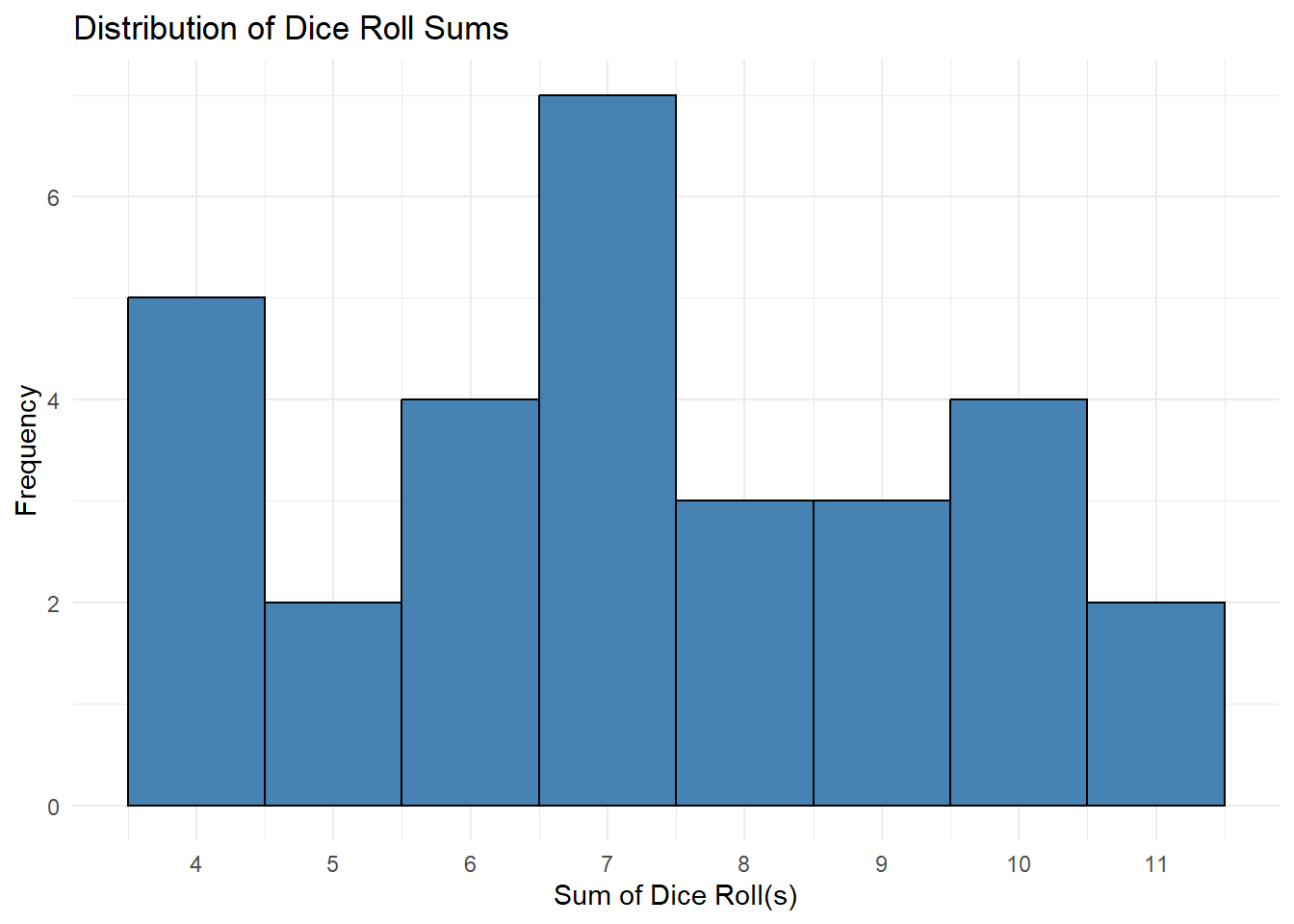

Now repeat the process with two dice. Add a histogram plotting the number of occurrences of each value like:

  results <- replicate(30, sum(sample(1:6, 2, replace = TRUE)))
  df <- data.frame(Draw = 1:30, Value = results)
ggplot(df, aes(x = Value)) +
    geom_histogram(binwidth = 1, fill = "steelblue", color = "black") +
    scale_x_continuous(breaks = seq(2, 6 * 2, 1)) +
    labs(
      title = "Distribution of Dice Roll Sums",
      x = "Sum of Dice Roll(s)",
      y = "Frequency"
    ) +
    theme_minimal()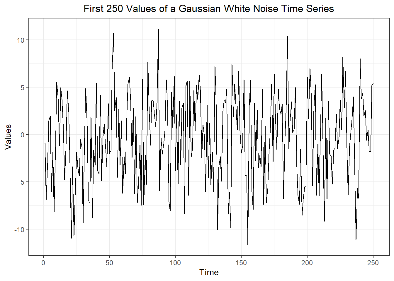

TipCheck Your Understanding

• Draw a histogram of the expected distribution. How does your results differ?
• What do you expect would happen if you rolled the 2 dice 5000 times?
• Is the process of rolling 2 dice a discrete white noise process?

Simulation

The following simulation illustrates a white noise time series.

TipCheck Your Understanding

• What do you notice about this time series?
• What characteristics do you observe in the correlogram?

Type I Errors

In your introductory statistics course, you probably learned about Type I error. Here is a quick refresher.

NoteType I Errors

Suppose we will conduct a hypothesis test with a level of significance equal to \(\alpha = 0.05\). If the null hypothesis is true, there is a probability of 0.05 that we will reject the null hypothesis. Due to sampling variation, we will reject a true null hypothesis 5% of the time. We refer to this as making a Type I Error.

When we create a correlogram, we actually conduct one hypothesis test for each value of \(k\). With so many hypothesis tests, it is not surprising if some of them show a significant correlation due to chance alone. In this case, we tend to disregard correlations that are barely significant and inexplicable.

TipCheck Your Understanding

Do the following with a partner:

1. Click on the [Simulate!] button above to generate a new simulated realization of the DWN process.
2. Out of the 20 autocorrelations represented in the correlogram, count the number that are statistically significant.
3. Repeat Steps 1. and 2. ten times, so you will have displayed 200 autocorrelations.

• What percentage of your autocorrelations were statistically significant?
• Compare your results with other teams.
• What percentage of these would you expect to be statistically significant, assuming the true autocorrelations are all zero?

Visualizing White Noise

# Set random seed
set.seed(10)

# Specify means and standard deviation
n <- 2500                           # number of points
white_noise_sigma <- rnorm(1, 5, 1) # choose a random standard deviation

# White noise data
white_noise_df <- data.frame(x = rnorm(n, 0, white_noise_sigma))

The first 250 points in this time series are illustrated here:

white_noise_df |> 
  mutate(t = 1:nrow(white_noise_df)) |>
  head(250) |>  
  ggplot(aes(x = t, y = x)) + 
    geom_line() +
    theme_bw() +
    labs(
      x = "Time",
      y = "Values",
      title = "First 250 Values of a Gaussian White Noise Time Series"
    ) +
    theme(
      plot.title = element_text(hjust = 0.5)
    )

Here is a histogram of the 2500 values from this DWN distribution.

white_noise_df |>
  mutate(density = dnorm(x, mean(white_noise_df$x), sd(white_noise_df$x))) |>
  ggplot(aes(x = x)) +
    geom_histogram(aes(y = after_stat(density)),
        color = "white", fill = "#56B4E9", binwidth = 1) +
    geom_line(aes(x = x, y = density)) +
    theme_bw() +
    labs(
      x = "Values",
      y = "Frequency",
      title = "Histogram of Values from a Gaussian White Noise Process"
    ) +
    theme(
      plot.title = element_text(hjust = 0.5)
    )

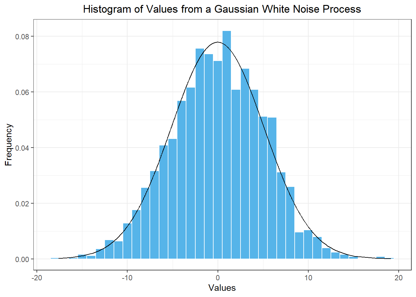
Notice that the values follow a normal distribution. This suggests the data are from a Gaussian white noise distribution.

Second-Order Properties of Discrete White Noise

When we refer to the second-order properties of a time series, we are talking about its variance and covariance. The mean is a first-order property, the covariance is a second-order property.

NoteSecond-Order Properties of a Discrete White Noise Process

If \(\{w_t\}_{t=1}^n\) is a DWN time series, then the population has the following properties.

\[ \mu_w = 0 \] and \[ cov(w_t, w_{t+k}) = \begin{cases} \sigma^2, & k = 0 \\ 0, & k \ne 0 \end{cases} \] The correlation function is therefore

\[ \rho_k = \begin{cases} 1, & k = 0 \\ 0, & k \ne 0 \end{cases} \]

Note that the properties given above are theoretical properties of the population, not estimates computed using a sample. The sample autocorrelations will not equal zero, due to randomness inherent in sampling.

Fitting the White Noise Model

Typically, a DWN series arises in the random component of another time series. If we have fully explained the level and seasonality in the time series, then the only component left is the random component, which would ideally follow a DWN process.

NoteIdentifying of a Discrete White Noise Process

A DWN process will have the following properties:

• There is a discrete observations.
• The mean of the observations is zero.
• The variance of the observations is finite.
• Successive observations are uncorrelated.

Since the mean of a DWN time series is zero, the only parameter we need to fit is the variance.

TipCheck Your Understanding

• Compute the sample variance for the DWN data in the file white_noise.parquet.

Class Activity: Random Walks (15 min)

Definitions

Consider moving on a number line, where your movements are determined by a discrete white noise (DWN) process. Each successive value indicates how far you will move along the number line from your current position. This is mathematically equivalent to allowing your position at time \(t\) to be the sum of all the observed DWN values up to time \(t\).

NoteDefinition of a Random Walk

Let \(\{x_t\}\) be a time series. Then, \(\{x_t\}\) is a random walk if it can be expressed as \[ x_{t} = x_{t-1} + w_{t} \] where \(\{w_t\}\) is a random process.

The value \(x_t\) can be considered as the cumulative summation of the first \(t\) values of the \(w_t\) series. In many cases, \(w_t\) is a discrete white noise series, and it is often modeled as a Gaussian white noise series. However, \(w_t\) could be as simple as a coin toss, as illustrated in the next activity.

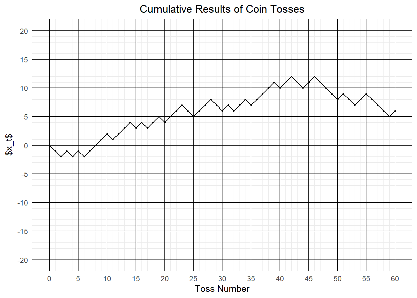
Simulating a Random Walk

In this activity, we will simulate a discrete-time, discrete-space random walk.

Do the following:

1. Start the time series at \(x_0 = 0\).

2. Toss a coin.

   • If the coin shows heads, then \(x_t = x_{t-1}+1\)
   • If the coin shows tails, then \(x_t = x_{t-1}-1\)

3. Plot the new point on the time plot.

4. Complete steps 2 and 3 a total of \(n=60\) times. (One realization is illustrated below.)

TipCheck Your Understanding

• How would you describe a random walk to someone who has not taken this class?
• How is a random walk related to a discrete white noise (DWN) process?
• Give a real-world example of a process that could be modeled by a random walk.

Representations for a Random Walk

Recall the definition of a random walk:

\(\{x_t\}\) is a random walk if it can be expressed as \[ x_{t} = x_{t-1} + w_{t} \] where \(\{w_t\}\) is a white noise series.

TipCheck Your Understanding

There are other ways to represent a random walk.

• Notice that \[\begin{align*} x_{t} &= x_{t-1} + w_{t} \\ x_{t-1} &= x_{t-2} + w_{t-1} \\ ⋮ ~~~ & ~~~~~~~~~~~~~~~ ⋮ \end{align*}\] Use this to write \(x_t\) in terms of \(x_{t-2}\), \(w_t\), and \(w_{t-1}\).

• Write \(x_t\) in terms of \(x_{t-3}\), \(w_t\), \(w_{t-1}\), and \(w_{t-2}\).

• Explain why it is possible to write \(x_t\) as \[ x_{t} = \sum\limits_{i=-\infty}^{t} w_{i} = w_{t} + w_{t-1} + w_{t-2} + w_{t-3} + \cdots \] where \(\{w_t\}\) is a DWN time series.

  Note that if the random walk is finite, we can write \(x_t\) as: \[ x_{t} = w_1 + w_2 + w_3 + \cdots + w_{t-3} + w_{t-2} + w_{t-1} + w_{t} \] where \(x_1=w_1\).

Class Activity: Backward Shift Operator (10 min)

Definition of the Backward Shift Operator

This process of back substitution is so common, we define notation to handle it.

NoteDefinition of the Backward Shift Operator

We define the backward shift operator or the lag operator, \(\mathbf{B}\), as: \[ \mathbf{B} x_t = x_{t-1} \] where \(\{x_t\}\) is any time series.

We can apply this operator repeatedly. We will use exponential notation to indicate this.

\[ \mathbf{B}^2 x_t = \mathbf{B} \mathbf{B} x_t = \mathbf{B} ( \mathbf{B} x_t ) = \mathbf{B} x_{t-1} = x_{t-2} \]

In general, \[ \mathbf{B}^n x_t = \underbrace{\mathbf{B} \cdot \mathbf{B} \cdot \cdots \cdot \mathbf{B}}_{n ~ \text{terms}} x_t = \mathbf{B}^{n-1} ( \mathbf{B} x_t ) = \mathbf{B}^{n-1} ( x_{t-1} ) = \mathbf{B}^{n-2} ( x_{t-2} ) = \cdots = \mathbf{B} x_{t-(n-1)} = x_{t-n} \]

Properties of the Backshift Operator

The backwards shift operator is a linear operator. So, if \(a\), \(b\), \(c\), and \(d\) are constants, then \[ (a \mathbf{B} + b)x_t = a \mathbf{B} x_t + b x_t \] The distributive property also holds. \[\begin{align*} (a \mathbf{B} + b)(c \mathbf{B} + d) x_t &= c (a \mathbf{B} + b) \mathbf{B} x_t + d(a \mathbf{B} + b) x_t \\ &= a \mathbf{B} (c \mathbf{B} + d) x_t + b (c \mathbf{B} + d) x_t \\ &= \left( ac \mathbf{B}^2 + (ad+bc) \mathbf{B} + bd \right) x_t \\ &= ac \mathbf{B}^2 x_t + (ad+bc) \mathbf{B} x_t + (bd) x_t \end{align*}\]

We will practice applying this operator.

TipCheck Your Understanding

Let \(\{x_t\}\) be a time series with the following values.

\(x_{1} = 5\),\(~\) \(x_{2} = 10\),\(~\) \(x_{3} = 13\),\(~\) \(x_{4} = 8\),\(~\) \(x_{5} = 4\),\(~\) \(x_{6} = 3\),\(~\) \(x_{7} = 9\),\(~\) \(x_{8} = 2\)

Evaluate the following.

• \(\mathbf{B} x_8\)
• \(\mathbf{B}^5 x_8\)
• \((\mathbf{B}^5 - \mathbf{B} ) x_8\)
• \(( \mathbf{B}^2 - 6 \mathbf{B} + 9 ) x_8\)
• \(( (\mathbf{B} - 6 )\mathbf{B} + 9 ) x_8\)
• \(( \mathbf{B} - 3 )^2 x_8 = ( \mathbf{B} - 3 ) \left[ ( \mathbf{B} - 3 ) x_8 \right]\)
• \(( 1 - \frac{1}{2} \mathbf{B} - \frac{1}{4} \mathbf{B}^2 - \frac{1}{8} \mathbf{B}^3 ) x_8\)

Class Activity: Properties of Random Walks (5 min)

Simulation

The following simulation illustrates a random walk.

TipCheck Your Understanding

• What do you notice about this time series?
• What characteristics do you observe in the correlogram?
• How does this compare to the time series and correlogram for the DWN process?

Second-Order Properties of a Random Walk

The second-order properties of a random walk are summarized below.

NoteSecond-Order Properties of a Random Walk

If \(\{x_t\}_{t=1}^n\) is a random walk, then the population has the following properties.

\[ \mu_x = 0 \] and \[ cov(x_t, x_{t+k}) = t \sigma^2 \]

TipClick here for a proof of the equation for \(cov(x_t,x_{t+k})\)

Why is \(cov(x_t, x_{t+k}) = t \sigma^2\)?

First, note that that since the terms in the white noise series are independent,

\[ cov ( w_i, w_j ) = \begin{cases} \sigma^2, & \text{if } ~ i=j \\ 0, & \text{otherwise} \end{cases} \]

Also, when random variables are independent, the covariance of a sum is the sum of the covariance.

Hence, \[\begin{align*} cov(x_t, x_{t+k}) &= cov ( \sum_{i=1}^t w_i, \sum_{j=1}^{t+K} w_j ) \\ &= \sum_{i=j} cov ( w_i, w_j ) \\ &= \sum_{i=1}^t \sigma^2 \\ &= t \sigma^2 \end{align*}\]

If \(k>0\) and \(t>0\), the correlation function is

\[ \rho_k = \frac{ cov(x_t, x_{t+k}) }{ \sqrt{var(x_t)} \sqrt{var(x_{t+k})} } = \frac{t \sigma^2}{\sqrt{t \sigma^2} \sqrt{(t+k) \sigma^2}} = \frac{1}{\sqrt{1+\frac{k}{t}}} \]

Note that the covariance of a random walk process depends on \(t\). Hence, random walks are non-stationary. The variance is unbounded as \(t\) increases. That implies a random walk will not provide good predictions in the long term.

Note that if \(0 < k \ll t\), then \(\rho_k \approx 1\). Because of this, a correlogram for a random walk will typically demonstrate positive autocorrelations that start near 1 and slowly decrease as \(k\) increases. This is exactly what we observed in the simulation above.

Homework Preview (5 min)

• Review upcoming homework assignment
• Clarify questions

NoteDownload Homework

homework_4_1.qmd

White Noise

The sample variance of the DWN data is computed using the R command var(white_noise_df$x) as 26.29.

Backward Shift Operator

\(x_{1} = 5\),\(~\) \(x_{2} = 10\),\(~\) \(x_{3} = 13\),\(~\) \(x_{4} = 8\),\(~\) \(x_{5} = 4\),\(~\) \(x_{6} = 3\),\(~\) \(x_{7} = 9\),\(~\) \(x_{8} = 2\)

Check Your Understanding Solutions: . - \(\mathbf{B} x_8 = x_7 = 9\) - \(\mathbf{B}^5 x_8 = x_3 = 13\) - \((\mathbf{B}^5 - \mathbf{B} ) x_8 = x_3 - x_7 = 13 - 9 = 4\) - \(( \mathbf{B}^2 - 6 \mathbf{B} + 9 ) x_8 = x_6 - 6 (x_7) + 9 (x_{t}) = 3 - 6 (9) + 9 (2) = -33\) - \(( (\mathbf{B} - 6) \mathbf{B} + 9 ) x_8 = -33\) - \(( \mathbf{B} - 3 )^2 x_8 = -33\) - \(( 1 - \frac{1}{2} B - \frac{1}{4} B^2 - \frac{1}{8} B^3 ) x_8 = x_8 - \frac{1}{2} x_7 - \frac{1}{4} x_6 - \frac{1}{8} x_5 = 2 - \frac{1}{2} (9) - \frac{1}{4} (3) - \frac{1}{8} (4) = -3.75\)