Fitted AR Models

Chapter 4: Lesson 4

Learning Outcomes

Fit time series models to data and interpret fitted parameters

Fit an $AR(p)$ model to simulated data
Explain the difference between parameters of the data generating process and estimates
Calculate confidence intervals for AR coefficient estimates
Interpret AR coefficient estimates in the context of the source and nature of historical data

Check model adequacy using diagnostic plots like correlograms of residuals

Compare AR fitted models to an underlying data generating process
Explain the limitations of stochastic model fitting as evidence in favor or against real world arguments.

Preparation

Read Sections 4.6-4.7

Learning Journal Exchange (10 min)

Review another student’s journal
What would you add to your learning journal after reading another student’s?
What would you recommend the other student add to their learning journal?
Sign the Learning Journal review sheet for your peer

Class Activity: Fitting a Simulated $AR(1)$ Model with Zero Mean (5 min)

We will demonstrate how AR models are fitted via simulation. We will fit two different $AR(1)$ models and an $AR(2)$ model. The advantage of using simulation is that we know how the time series was constructed. So, we know the model that was used and the actual values of the parameters in that model. We can then see how close our estimated parameter values are to the true values.

Simulate an $AR(1)$ Time Series

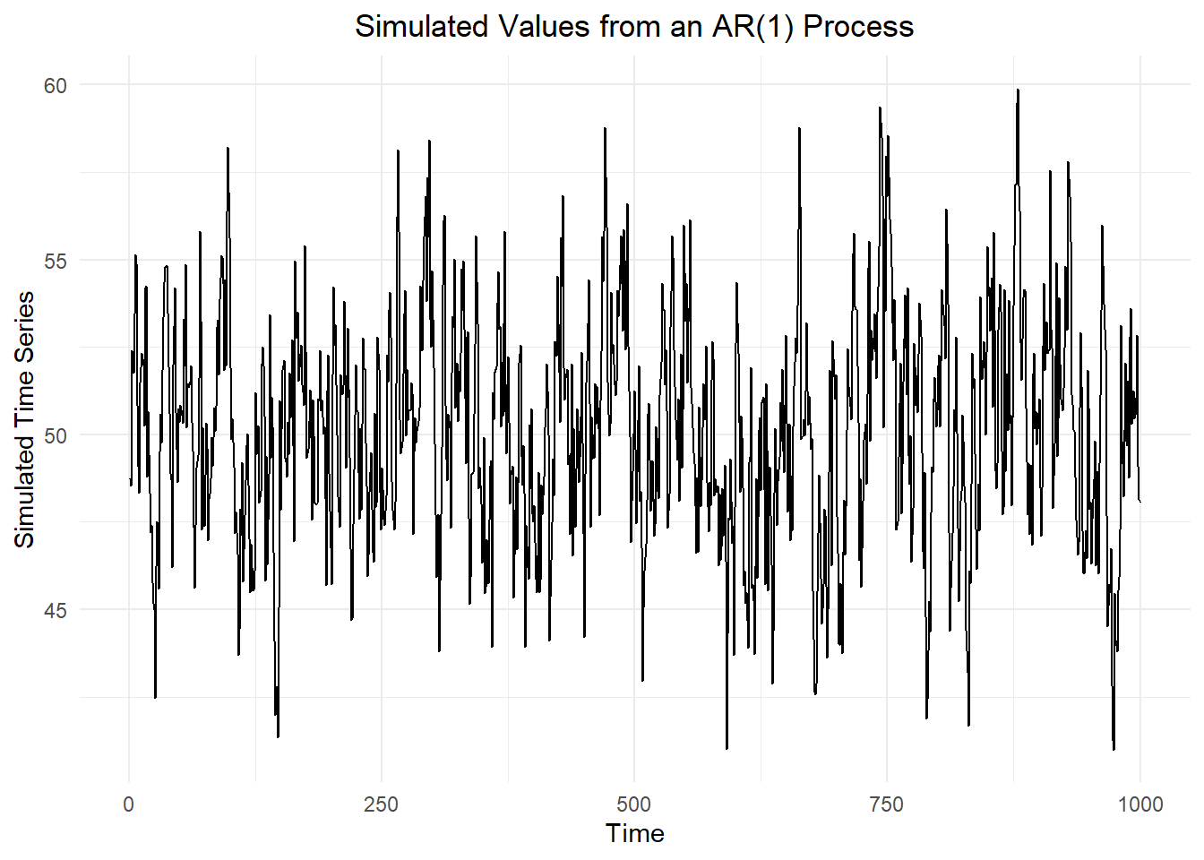
In this simulation, we first simulate data from the $AR(1)$ model \[ x_t = 0.75 ~ x_{t-1} + w_t \] where $w_t$ is a white noise process with variance 1.

Show the code

set.seed(123)
n_rep <- 1000
alpha1 <- 0.75

dat_ts <- tibble(w = rnorm(n_rep)) |>
  mutate(
    index = 1:n(),
    x = purrr::accumulate2(
      lag(w), w, 
      \(acc, nxt, w) alpha1 * acc + w,
      .init = 0)[-1]) |>
  tsibble::as_tsibble(index = index)

dat_ts |> 
  autoplot(.vars = x) +
    labs(
      x = "Time",
      y = "Simulated Time Series",
      title = "Simulated Values from an AR(1) Process"
    ) +
    theme_minimal() +
    theme(
      plot.title = element_text(hjust = 0.5)
    )

The R command mean(dat_ts$x) gives the mean of the $x_t$ values as 0.067.

Fit an $AR(1)$ Model with Zero Mean

Show the code

# Fit the AR(1) model
fit_ar <- dat_ts |>
  model(AR(x ~ order(1)))
tidy(fit_ar)

# A tibble: 1 × 6
  .model           term  estimate std.error statistic   p.value
  <chr>            <chr>    <dbl>     <dbl>     <dbl>     <dbl>
1 AR(x ~ order(1)) ar1      0.720    0.0220      32.8 2.07e-160

The estimate of the parameter $\alpha_1$ (i.e. the fitted value of the parameter $\alpha_1$) is $\hat \alpha_1 = 0.72$.

When R fits an AR model, the mean of the time series is subtracted from the data before the parameter values are estimated. If R detects that the mean of the time series is not significantly different from zero, it is omitted from the output.

Because the mean is subtracted from the time series before the parameter values are estimated, R is using the model \[ z_t = \alpha_1 ~ z_{t-1} + w_t \] where $z_t = x_t - \mu$ and $\mu$ is the mean of the time series.

Check Your Understanding

Answer the following questions with your partner.

Use the expression for $z_t$ above to solve for $x_t$ in terms of $x_{t-1}$, $\mu$, $\alpha_1$, and $w_t$.
What does your model reduce to when $\mu = 0$?
Explain to your partner why this correctly models a time series with mean $\mu$.

We replace the parameter $\mu$ with its estimator $\hat \mu = \bar x$. We also replace $\alpha_1$ with the fitted value from the output $\hat \alpha_1$. This gives us the fitted model: \[ \hat x_t = \bar x + \hat \alpha_1 ~ (x_{t-1} - \bar x) \]

The fitted model can be expressed as:

\[\begin{align*} \hat x_t &= 0.067 + 0.72 \left( x_{t-1} - 0.067 \right) \\ &= 0.067 - 0.72 ~ (0.067) + 0.72 ~ \left( x_{t-1} \right) \\ &= 0.019 + 0.72 ~ x_{t-1} \end{align*}\]

Even though R does not report the parameter for the mean of the process, $\hat \mu = 0.019$, it is not significantly different from zero. One could argue that we should not use a model that contains the mean and instead focus on a simple fitted model that has only one parameter:

\[ \hat x_t = 0.72 ~ x_{t-1} \]

Confidence Interval for the Model Parameter

The P-value given above tests the hypothesis that $\alpha_1=0$. This is not helpful in this context. We are interested in the plausible values for $\alpha_1$, not whether or not it is different from zero. For this reason, we consider a confidence interval and disregard the P-value.

We can compute an approximate 95% confidence interval for $\alpha_1$ as: \[ \left( \hat \alpha_1 - 2 \cdot SE_{\hat \alpha_1} , ~ \hat \alpha_1 + 2 \cdot SE_{\hat \alpha_1} \right) \] where $\hat \alpha_1$ is our parameter estimate and $SE_{\hat \alpha_1}$ is the standard error of the estimate. Both of these values are given in the R output.

Show the code

ci_summary <- tidy(fit_ar) |>
    mutate(
        lower = estimate - 2 * std.error,
        upper = estimate + 2 * std.error
    )

So, our 95% confidence interval for $\alpha_1$ is: \[ \left( 0.72 - 2 \cdot 0.022 , ~ 0.72 + 2 \cdot 0.022 \right) \] or \[ \left( 0.676 , ~ 0.764 \right) \] Note that the confidence interval contains $\alpha_1 = 0.75$, the value of the parameter we used in our simulation. The process of estimating the parameter worked well. In practice, we will not know the value of $\alpha_1$, but the confidence interval gives us a reasonable estimate of the value.

Residuals

For an $AR(1)$ model where the mean of the time series is not statistically significantly different from 0, the residuals are computed as \[\begin{align*} r_t &= x_t - \hat x_t \\ &= x_t - \left[ 0.72 ~ x_{t-1} \right] \end{align*}\]

We can easily obtain these residual values in R:

The variance of the residuals is $0.982$. This is very close to the actual value used in the simulation: $\sigma^2 = 1$.

Class Activity: Fitting a Simulated $AR(1)$ Model with Non-Zero Mean (5 min)

Simulate an $AR(1)$ Time Series

It is easy to conceive situations where the mean of an AR model, $\mu$, is not zero. The model we have been fitting is \[ x_t = \mu + \alpha_1 ~ \left( x_{t-1} - \mu \right) + w_t \] where $\mu$ and $\alpha_1$ are constants, and $w_t$ is a white noise process with variance $\sigma^2$.

This model can be simplified by combining like terms. \[\begin{align*} x_t &= \mu + \alpha_1 ~ \left( x_{t-1} - \mu \right) + w_t \\ &= \underbrace{\mu - \alpha_1 ~ (\mu)}_{\alpha_0} + \alpha_1 ~ \left( x_{t-1} \right) + w_t \\ &= \alpha_0 + \alpha_1 ~ \left( x_{t-1} \right) + w_t \end{align*}\]

Suppose the mean of the $AR(1)$ process is $\mu = 50$. We will set $\alpha_1 = 0.75$, and $\sigma^2 = 5$ for this simulation. After specifying these numbers, the model becomes: \[\begin{align*} x_t &= 50 + 0.75 ~ ( x_{t-1} - 50 ) + w_t \\ &= 50 - 0.75 ~ ( 50 ) + 0.75 ~ x_{t-1} + w_t \\ &= 12.5 + 0.75 ~ x_{t-1} + w_t \end{align*}\] where $w_t$ is a white noise process with variance $\sigma^2 = 5$.

Show the code

set.seed(123)
n_rep <- 1000
alpha1 <- 0.75
sigma_sqr <- 5

dat_ts <- tibble(w = rnorm(n = n_rep, sd = sqrt(sigma_sqr))) |>
  mutate(
    index = 1:n(),
    x = purrr::accumulate2(
      lag(w), w, 
      \(acc, nxt, w) alpha1 * acc + w,
      .init = 0)[-1]) |>
  mutate(x = x + alpha0) |> 
  tsibble::as_tsibble(index = index)

dat_ts |> 
  autoplot(.vars = x) +
    labs(
      x = "Time",
      y = "Simulated Time Series",
      title = "Simulated Values from an AR(1) Process"
    ) +
    theme_minimal() +
    theme(
      plot.title = element_text(hjust = 0.5)
    )

The R command mean(dat_ts$x) gives the mean of the $x_t$ values as 50.15.

Fit an $AR(1)$ Model with Non-Zero Mean

We now use R to fit an $AR(1)$ model to the time series data.

Show the code

# Fit the AR(1) model
fit_ar <- dat_ts |>
  model(AR(x ~ order(1)))
tidy(fit_ar)

# A tibble: 2 × 6
  .model           term     estimate std.error statistic   p.value
  <chr>            <chr>       <dbl>     <dbl>     <dbl>     <dbl>
1 AR(x ~ order(1)) constant   14.1      1.11        12.7 1.35e- 34
2 AR(x ~ order(1)) ar1         0.719    0.0220      32.7 5.95e-160

The estimate of the parameter for the constant (mean) term $\alpha_0$ is $\hat \alpha_0 = 14.091$. The estimate of the parameter $\alpha_1$ (i.e. the fitted value of the parameter $\alpha_1$) is $\hat \alpha_1 = 0.719$.

Fitting the model \[ x_t = \alpha_0 + \alpha_1 ~ x_{t-1} + w_t \] we get \[\begin{align*} \hat x_t &= \hat \alpha_0 + \hat \alpha_1 ~ x_{t-1} \\ &= 14.091 + 0.719 ~ x_{t-1} \end{align*}\]

Confidence Intervals for the Model Parameters

We can compute approximate 95% confidence intervals for $\alpha_0$ and $\alpha_1$:

\[ \left( \hat \alpha_i - 2 \cdot SE_{\hat \alpha_i} , ~ \hat \alpha_i + 2 \cdot SE_{\hat \alpha_i} \right) \] where $\hat \alpha_i$ is our estimate of parameter $i \in \{0,1\}$, and $SE_{\hat \alpha_i}$ is the standard error of the respective estimates.

Show the code

ci_summary <- tidy(fit_ar) |>
    mutate(
        lower = estimate - 2 * std.error,
        upper = estimate + 2 * std.error
    )

95% Confidence Interval for $\alpha_0$: \[ \left( \hat \alpha_0 - 2 \cdot SE_{\hat \alpha_0} , ~ \hat \alpha_0 + 2 \cdot SE_{\hat \alpha_0} \right) \]

\[ \left( 14.091 - 2 \cdot 1.105 , ~ 14.091 + 2 \cdot 1.105 \right) \]

\[ \left( 11.88 , ~ 16.301 \right) \] The confidence interval for $\alpha_0$ contains \[\alpha_0 = \mu - \alpha_1 ~ (\mu) = 12.5\]

95% Confidence Interval for $\alpha_1$: \[ \left( \hat \alpha_1 - 2 \cdot SE_{\hat \alpha_1} , ~ \hat \alpha_1 + 2 \cdot SE_{\hat \alpha_1} \right) \]

\[ \left( 0.719 - 2 \cdot 0.022 , ~ 0.719 + 2 \cdot 0.022 \right) \]

\[ \left( 0.675 , ~ 0.763 \right) \] The confidence interval for $\alpha_1$ contains \[\alpha_1 = 0.75\]

Both intervals captured the true value used in the simulation. The process of estimating the parameter worked well. In practice, we will not know the value of $\alpha_1$, but the confidence interval gives us a reasonable estimate of the value. About 95% of the time, the confidence interval will capture the true parameter value.

Residuals

The residuals in this model are computed as \[\begin{align*} r_t &= x_t - \hat x_t \\ &= x_t - \left[ 14.091 + 0.719 ~ x_{t-1} \right] \end{align*}\]

The variance of the residuals is $4.911$, which is near the actual parameter value: $\sigma^2 = 5$.

Class Activity: Fitting a Simulated $AR(2)$ Model (10 min)

Simulate an $AR(2)$ Time Series

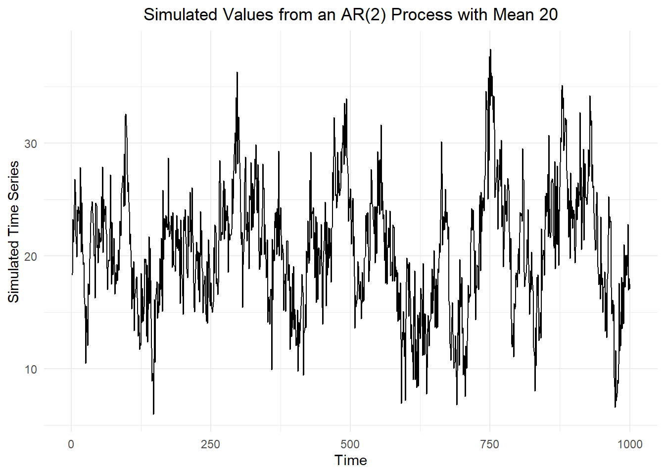
In this section, we will simulate data from the following $AR(2)$ process: \[ x_t = 2 + 0.5 ~ x_{t-1} + 0.4 ~ x_{t-2} + w_t \] where $w_t$ is a discrete white noise process with variance $\sigma^2 = 9$.

Check Your Understanding

Use the $AR(2)$ process above to answer the following questions.

Is this $AR(2)$ process stationary? (Hint: The characteristic polynomial only includes terms that involve $x_t$.)
Rewrite the model in the form \[ x_t = \mu + \alpha_1 ~ ( x_{t-1} - \mu) + \alpha_2 ~ ( x_{t-2} - \mu) + w_t \] Identify the value of each of the coefficients ($\mu$, $\alpha_1$, and $\alpha_2$).
What is the mean of this $AR(2)$ process?

Here is a time plot of the simulated time series.

Show the code

set.seed(123)
n_rep <- 1000
alpha0 <- 20
alpha1 <- 0.5
alpha2 <- 0.4
sigma_sqr <- 9

dat_ts <- tibble(w = rnorm(n = n_rep, sd = sqrt(sigma_sqr))) |>
    mutate(
      index = 1:n(),
      x = 0
    ) |>
    tsibble::as_tsibble(index = index)

# Simulate x values
dat_ts$x[1] <- alpha0 + dat_ts$w[1]
dat_ts$x[2] <- alpha0 + alpha1 * ( dat_ts$x[1] - alpha0 ) + dat_ts$w[2]
for (i in 3:nrow(dat_ts)) {
  dat_ts$x[i] <- alpha0 + 
    alpha1 * ( dat_ts$x[i-1] - alpha0 ) + 
    alpha2 * ( dat_ts$x[i-2] - alpha0 ) + 
    dat_ts$w[i]
}

dat_ts |> 
  autoplot(.vars = x) +
    labs(
      x = "Time",
      y = "Simulated Time Series",
      title = paste("Simulated Values from an AR(2) Process with Mean", alpha0)
    ) +
    theme_minimal() +
    theme(
      plot.title = element_text(hjust = 0.5)
    )

Fit an $AR(2)$ Model

We fit an $AR(2)$ model to these simulated values.

Show the code

# Fit the AR(2) model
fit_ar <- dat_ts |>
    model(AR(x ~ order(2))) 
tidy(fit_ar)

# A tibble: 3 × 6
  .model           term     estimate std.error statistic  p.value
  <chr>            <chr>       <dbl>     <dbl>     <dbl>    <dbl>
1 AR(x ~ order(2)) constant    2.33     0.380       6.14 1.17e- 9
2 AR(x ~ order(2)) ar1         0.478    0.0289     16.5  1.75e-54
3 AR(x ~ order(2)) ar2         0.408    0.0289     14.1  1.96e-41

The estimates of the parameter values are:
$\hat \alpha_0 = 2.333$, $\hat \alpha_1 = 0.478$, and $\hat \alpha_2 = 0.408$. This means that our fitted model can be expressed as:

\[\begin{align*} \hat x_t &= \hat \alpha_0 + \hat \alpha_1 ~ x_{t-1} + \hat \alpha_2 ~ x_{t-2} \\ &= 2.333 + 0.478 ~ x_{t-1} + 0.408 ~ x_{t-2} \end{align*}\]

Confidence Interval for the Model Parameters

We can compute an approximate 95% confidence interval for $\alpha_i$ as: \[ \left( \hat \alpha_i - 2 \cdot SE_{\hat \alpha_i} , ~ \hat \alpha_i + 2 \cdot SE_{\hat \alpha_i} \right) \] where $\hat \alpha_i$ is our estimate of the $i^{th}$ parameter and $SE_{\hat \alpha_i}$ is the standard error of the respective estimate. These values are given in the R output from the code below.

Show the code

ci_summary <- tidy(fit_ar) |>
    mutate(
        lower = estimate - 2 * std.error,
        upper = estimate + 2 * std.error
    )

95% confidence interval for $\alpha_0$: \[ \left( \hat \alpha_0 - 2 \cdot SE_{\hat \alpha_0} , ~ \hat \alpha_0 + 2 \cdot SE_{\hat \alpha_0} \right) \] \[ \left( 2.333 - 2 \cdot 0.38 , \right. ~~~~~~~~~~~~~~~~~~~ \] \[ ~~~~~~~~~~~~~~~~~~~ \left. 2.333 + 2 \cdot 0.38 \right) \] \[ \left( 1.574 , ~ 3.093 \right) \] This confidence interval contains $\alpha_0 = 2$.

95% confidence interval for $\alpha_1$: \[ \left( \hat \alpha_1 - 2 \cdot SE_{\hat \alpha_1} , ~ \hat \alpha_1 + 2 \cdot SE_{\hat \alpha_1} \right) \] \[ \left( 0.478 - 2 \cdot 0.029 , \right. ~~~~~~~~~~~~~~~~~~~ \] \[ ~~~~~~~~~~~~~~~~~~~ \left. 0.478 + 2 \cdot 0.029 \right) \] \[ \left( 0.42 , ~ 0.536 \right) \] This confidence interval contains $\alpha_1 = 0.5$.

95% confidence interval for $\alpha_2$: \[ \left( \hat \alpha_2 - 2 \cdot SE_{\hat \alpha_2} , ~ \hat \alpha_2 + 2 \cdot SE_{\hat \alpha_2} \right) \] \[ \left( 0.408 - 2 \cdot 0.029 , \right. ~~~~~~~~~~~~~~~~~~~ \] \[ ~~~~~~~~~~~~~~~~~~~ \left. 0.408 + 2 \cdot 0.029 \right) \] \[ \left( 0.35 , ~ 0.466 \right) \] This confidence interval contains $\alpha_2 = 0.4$.

All three confidence intervals contain the true parameter values we used for the simulation.

Residuals

We can compute the residuals in the same manner as we did for the other models.

Check Your Understanding

Working with a partner, do the following

Write the expression used to compute the residuals.
Find the residuals of this sequence using your expression.
Here are the first few residuals. Compare these to the values you computed.

Show the code

fit_ar |>
  residuals()

# A tsibble: 1,000 x 3 [1]
# Key:       .model [1]
   .model           index .resid
   <chr>            <int>  <dbl>
 1 AR(x ~ order(2))     1 NA    
 2 AR(x ~ order(2))     2 NA    
 3 AR(x ~ order(2))     3  4.60 
 4 AR(x ~ order(2))     4  0.237
 5 AR(x ~ order(2))     5  0.330
 6 AR(x ~ order(2))     6  5.13 
 7 AR(x ~ order(2))     7  1.46 
 8 AR(x ~ order(2))     8 -3.78 
 9 AR(x ~ order(2))     9 -2.13 
10 AR(x ~ order(2))    10 -1.39 
# ℹ 990 more rows

Explain why there are no residuals for times $t=1$ and $t=2$.

The variance of the residuals is 8.857. This is close to 9, the parameter used in the simulation.

Small-Group Activity: Global Warming (20 min)

The time plot below illustrates the change in global surface temperature compared to the long-term average observed from 1951 to 1980. (Source: NASA/GISS.)

Show the code

temps_ts <- rio::import("https://byuistats.github.io/timeseries/data/global_temparature.csv") |>
  as_tsibble(index = year)

temps_ts |> autoplot(.vars = change) +
    labs(
      x = "Year",
      y = "Temperature Change (Celsius)",
      title = paste0("Change in Mean Annual Global Temperature (", min(temps_ts$year), "-", max(temps_ts$year), ")")
    ) +
    theme_minimal() +
    theme(
      plot.title = element_text(hjust = 0.5)
    )

Using the PACF to Choose $p$ for an $AR(p)$ Process

In the previous lesson, we noted that the partial correlogram can be used to assess the number of parameters in an AR model. Here is a partial correlogram for the change in the mean annual global temperature.

Show the code

pacf(temps_ts$change)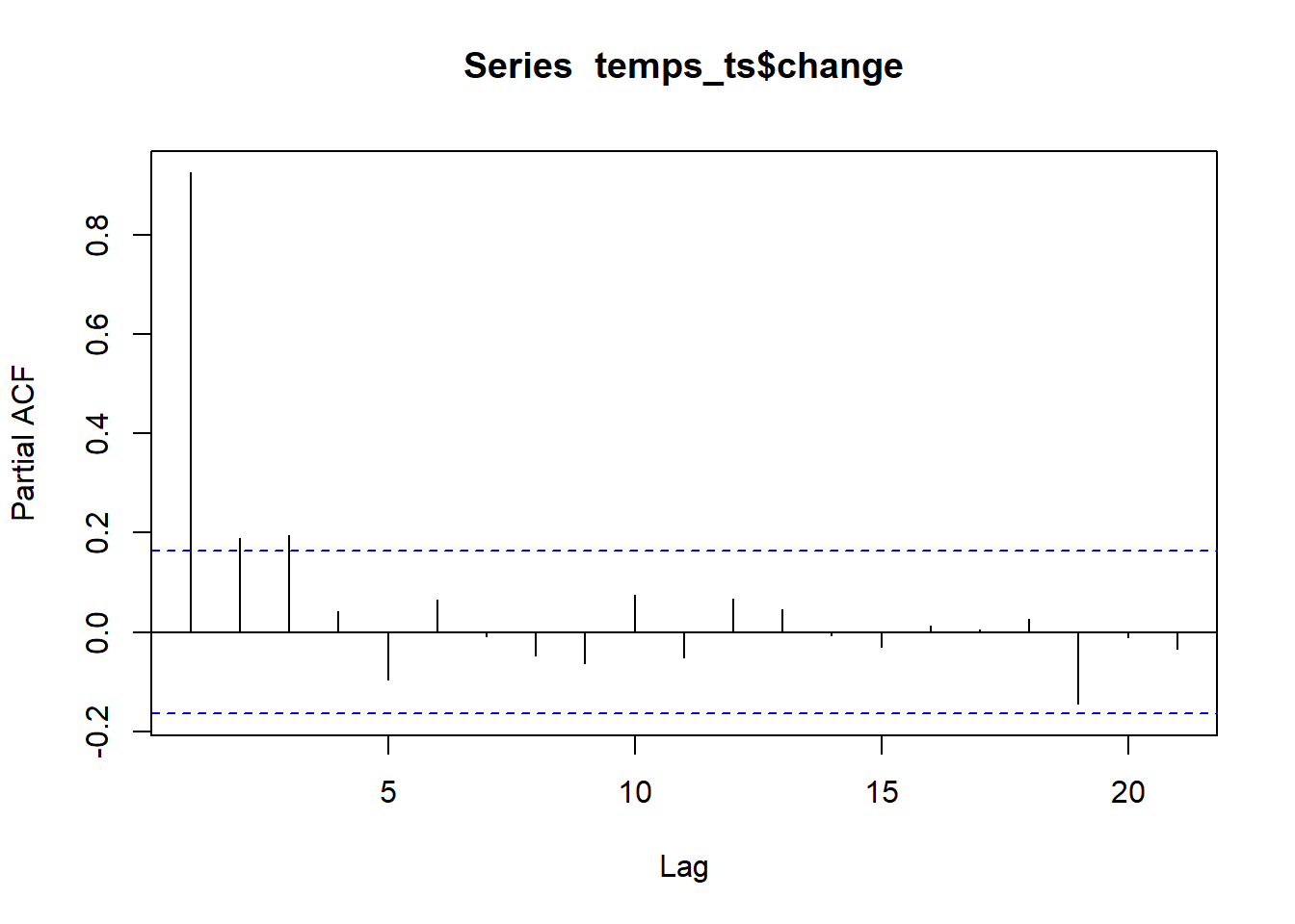

Check Your Understanding

Working with your partner, do the following:

We will apply an $AR(p)$ model. What value of $p$ is suggested by the pacf?
Using the value of $p$ you identified, fit an $AR(p)$ model to the global temperature data. State the fitted $AR(p)$ model in the form \[\hat x_t = \cdots\]
Obtain 95% confidence intervals for each of the parameters. Which are significantly different from zero?
Give the first three residual values (skipping the NAs).
What is the estimate of $\sigma^2$?
Make a correlogram for the residuals. Does it appear that your model has fully explained the variation in the temperatures?

Fitting Models (Dynamic Number of Parameters)

You may have concluded that $p=3$ might be insufficient for modeling these data. We now explore a technique that allows R to choose $p$ based on the significance of the parameters.

If we specify order(1:9) in the model statement, R returns the largest $AR(p)$ model (up to $p=9$) for which the parameter $\alpha_p$ is significant.

Show the code

global_ar <- temps_ts |>
    model(AR(change ~ order(1:9)))
tidy(global_ar)

# A tibble: 7 × 6
  .model                  term     estimate std.error statistic  p.value
  <chr>                   <chr>       <dbl>     <dbl>     <dbl>    <dbl>
1 AR(change ~ order(1:9)) constant   0.0190   0.00881     2.15  3.30e- 2
2 AR(change ~ order(1:9)) ar1        0.656    0.0841      7.80  1.40e-12
3 AR(change ~ order(1:9)) ar2       -0.0662   0.100      -0.659 5.11e- 1
4 AR(change ~ order(1:9)) ar3        0.140    0.0988      1.42  1.58e- 1
5 AR(change ~ order(1:9)) ar4        0.265    0.0995      2.67  8.58e- 3
6 AR(change ~ order(1:9)) ar5       -0.163    0.102      -1.60  1.11e- 1
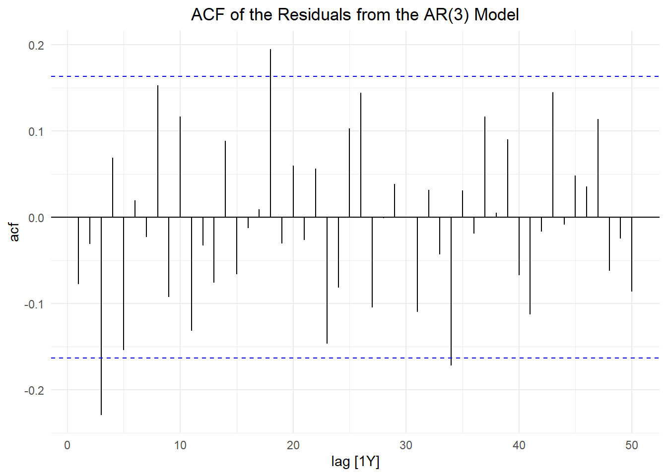
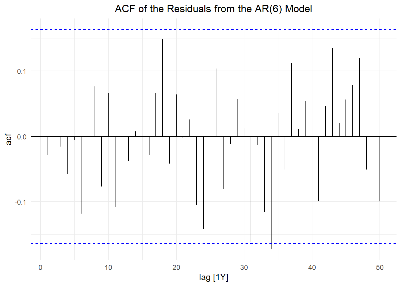
7 AR(change ~ order(1:9)) ar6        0.206    0.0863      2.38  1.85e- 2

R returned an $AR(6)$ model for this time series.

Check Your Understanding

Working with your partner, do the following:

State the fitted $AR(p)$ model in the form \[\hat x_t = \cdots\]
Obtain 95% confidence intervals for each of the parameters. Which are significantly different from zero?
Give the first three residual values (skipping the NAs).
What is the estimate of $\sigma^2$?
Make a correlogram for the residuals. Does it appear that your model has fully explained the variation in the temperatures? Justify your answer.

Stationarity of the $AR(p)$ Model

With the exception of a lone seemingly spurious autocorrelation, there are no significant values of the acf of the residuals in the $AR(6)$ model. This suggests that the model accounts for the variation in the time series.

Check Your Understanding

Write the characteristic equation for the $AR(6)$ model you developed.
Click on the link below to obtain a more precise version of the characteristic equation, then solve the characteristic equation by any method.

Characteristic Equation

Is our $AR(6)$ model stationary?

Class Activity: Forecasting with an $AR(p)$ Model (5 min)

We now use the model to forecast the mean temperature difference for the next 50 years.

Show the code

temps_forecast <- global_ar |> forecast(h = "50 years")
temps_forecast |>
  autoplot(temps_ts, level = 95) +
  geom_line(aes(y = .fitted, color = "Fitted"),
    data = augment(global_ar)) +
  scale_color_discrete(name = "") +
  labs(
    x = "Year",
    y = "Temperature Change (Celsius)",
    title = paste0("Change in Mean Annual Global Temperature (", min(temps_ts$year), "-", max(temps_ts$year), ")"),
    subtitle = paste0("50-Year Forecast Based on our AR(", tidy(global_ar) |> as_tibble() |> dplyr::select(term) |> tail(1) |> right(1), ") Model")
  ) +
  theme_minimal() +
  theme(
    plot.title = element_text(hjust = 0.5),
    plot.subtitle = element_text(hjust = 0.5)
  )

Check Your Understanding

Does this forecast seem appropriate for the data? Why or why not?

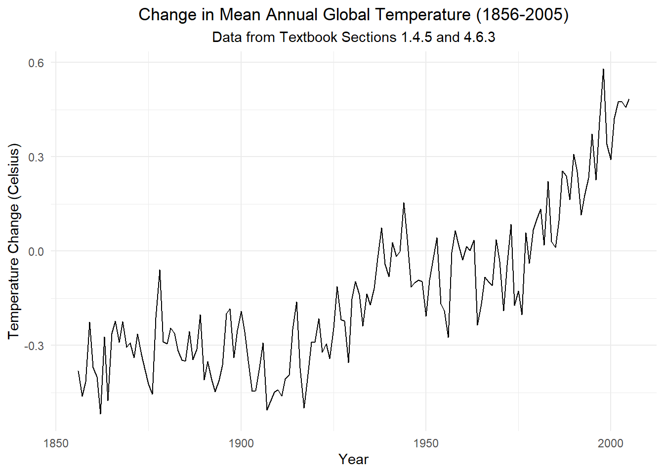
Class Activity: Comparison to the Results in Section 4.6.3 of the Book (5 min)

In Sections 1.4.5 and 4.6.3 of the textbook, the authors present a similar dataset on the mean annual temperatures on Earth through 2005. Here is a time plot of their data:

Show the code

global_ts <- tibble(x = scan("data/global.dat")) |>
  mutate(
        date = seq(
            ymd("1856-01-01"),
            by = "1 months",
            length.out = n()),
        year = year(date),
        year_month = tsibble::yearmonth(date)
  ) |>
  summarise(x = mean(x), .by = year) |>
  as_tsibble(index = year) 
global_ts |> autoplot(.vars = x) +
    labs(
      x = "Year",
      y = "Temperature Change (Celsius)",
      title = paste0("Change in Mean Annual Global Temperature (", min(global_ts$year), "-", max(global_ts$year), ")"),
      subtitle = "Data from Textbook Sections 1.4.5 and 4.6.3"
    ) +
    theme_minimal() +
    theme(
      plot.title = element_text(hjust = 0.5),
      plot.subtitle = element_text(hjust = 0.5)
    )

The fitted $AR(4)$ model is given below.

Show the code

global_ar_book <- global_ts |>
  model(AR(x ~ order(1:9)))
tidy(global_ar_book)

# A tibble: 4 × 6
  .model             term  estimate std.error statistic  p.value
  <chr>              <chr>    <dbl>     <dbl>     <dbl>    <dbl>
1 AR(x ~ order(1:9)) ar1     0.582     0.0791     7.36  1.24e-11
2 AR(x ~ order(1:9)) ar2     0.0216    0.0919     0.236 8.14e- 1
3 AR(x ~ order(1:9)) ar3     0.107     0.0917     1.17  2.43e- 1
4 AR(x ~ order(1:9)) ar4     0.267     0.0791     3.38  9.43e- 4

Let’s check the stationarity of this model. The characteristic equation is:

Show the code

alphas <- global_ar_book |> coefficients() |> dplyr::select(estimate) |> pull()
cat(
  "0 = 1", 
        "- (", alphas[1], ") * x",
        "- (", alphas[2], ") * x^2",
        "- (", alphas[3], ") * x^3",
        "- (", alphas[4], ") * x^4"
)

0 = 1 - ( 0.5817607 ) * x - ( 0.02164876 ) * x^2 - ( 0.1074731 ) * x^3 - ( 0.2670716 ) * x^4

The solutions of the characteristic equation are:

Show the code

polyroot(c(1, -alphas)) |> round(3)

[1]  1.011+0.000i -1.755+0.000i  0.171-1.443i  0.171+1.443i

The absolute value of the solutions of the characteristic equation are:

Show the code

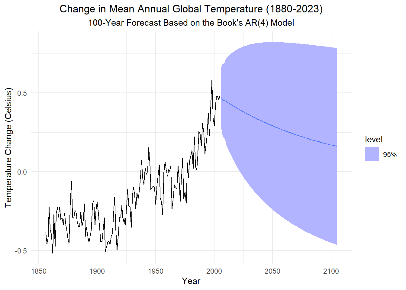
polyroot(c(1, -alphas)) |> abs() |> round(3)

[1] 1.011 1.755 1.453 1.453

Check Your Understanding

Is the textbook’s model stationary?
In the textbook, the author stated, “The correlogram of the residuals has only one (marginally) significant value at lag 27, so the underlying residual series could be white noise (Fig. 4.14). Thus the fitted AR(4) model (Equation (4.24)) provides a good fit to the data. As the AR model has no deterministic trend component, the trends in the data can be explained by serial correlation and random variation, implying that it is possible that these trends are stochastic (or could arise from a purely stochastic process). Again we emphasise that this does not imply that there is no underlying reason for the trends. If a valid scientific explanation is known, such as a link with the increased use of fossil fuels, then this information would clearly need to be included in any future forecasts of the series.”
- What is the author saying?
- How would you respond to this statement?

Here is a plot of the forecasted values for the next 100 years, based on the textbook’s model:

Show the code

# global_ar_book <- global_ts |>
#   model(AR(x ~ order(4)))
temps_forecast_book <- global_ar_book |> forecast(h = "100 years")
temps_forecast_book |>
  autoplot(global_ts, level = 95) +
#   geom_line(aes(y = .mean, color = "Fitted"),
#     data = augment(global_ar_book)) +
#   scale_color_discrete(name = "") +
    labs(
      x = "Year",
      y = "Temperature Change (Celsius)",
      title = paste0("Change in Mean Annual Global Temperature (", min(temps_ts$year), "-", max(temps_ts$year), ")"),
      subtitle = "100-Year Forecast Based on the Book's AR(4) Model"
    ) +
    theme_minimal() +
    theme(
      plot.title = element_text(hjust = 0.5),
      plot.subtitle = element_text(hjust = 0.5)
    )

Check Your Understanding

Compare and contrast the results you observed in the two global temperature time series.
What conclusions do you draw?

Homework Preview (5 min)

Review upcoming homework assignment
Clarify questions

Download Homework

homework_4_4.qmd

Small-Group Activity: Global Warming–PACF

Check Your Understanding

Working with your partner, do the following

We will apply an $AR(p)$ model. What value of $p$ is suggested by the pacf?

Solution:

\[p=3\]

Using the value of $p$ you identified, fit an $AR(p)$ model to the global temperature data. State the fitted $AR(p)$ model in the form \[\hat x_t = \cdots\]

Solution:

Show the code

global_ar <- temps_ts |>
    model(AR(change ~ order(3)))
tidy(global_ar)

# A tibble: 3 × 6
  .model                term  estimate std.error statistic  p.value
  <chr>                 <chr>    <dbl>     <dbl>     <dbl>    <dbl>
1 AR(change ~ order(3)) ar1     0.737     0.0823     8.95  1.80e-15
2 AR(change ~ order(3)) ar2    -0.0350    0.103     -0.339 7.35e- 1
3 AR(change ~ order(3)) ar3     0.319     0.0839     3.80  2.15e- 4

Note that the constant term is not statistically significant. If we ignore this term, we get the fitted model:

\[\begin{align*} \hat x_t &= 0 + \hat \alpha_1 ~ x_{t-1} + \hat \alpha_2 ~ x_{t-2} + \hat \alpha_3 ~ x_{t-3} \\ &= 0.737 ~ x_{t-1} + (-0.035) ~ x_{t-2} + 0.319 ~ x_{t-3} \end{align*}\]

If we want to incorporate the constant term in the model, then we need to find the mean of the time series. The mean of the time series is:

mean(temps_ts$change)

[1] 0.06923611

The fitted AR model is

\[\begin{align*} \hat x_t &= \hat \mu + \hat \alpha_1 ~ (x_{t-1} - \mu) + \hat \alpha_2 ~ (x_{t-2} - \mu) + \hat \alpha_3 ~ (x_{t-3} - \mu) \\ &= \underbrace{ \hat \mu - \hat \alpha_1 (\hat \mu) - \hat \alpha_2 (\hat \mu) - \hat \alpha_3 (\hat \mu) }_{\hat \alpha_0} + \hat \alpha_1 ~ x_{t-1} + \hat \alpha_2 ~ x_{t-2} + \hat \alpha_3 ~ x_{t-3} \\ &= \hat \alpha_0 + \hat \alpha_1 ~ x_{t-1} + \hat \alpha_2 ~ x_{t-2} + \hat \alpha_3 ~ x_{t-3} \end{align*}\] Or, after substituting the fitted values: \[\begin{align*} \hat x_t &= 0.069 + 0.737 ~ ( x_{t-1} - 0.069) + (-0.035) ~ ( x_{t-2} - 0.069) + 0.319 ~ ( x_{t-3} - 0.069) \\ &= -0.0014 + 0.737 ~ x_{t-1} + (-0.035) ~ x_{t-2} + 0.319 ~ x_{t-3} \end{align*}\]

Obtain 95% confidence intervals for each of the parameters. Which are significantly different from zero?

Solution:

Show the code

ci_summary <- tidy(global_ar) |>
    mutate(
        lower = estimate - 2 * std.error,
        upper = estimate + 2 * std.error
    )

The confidence intervals are: \[\begin{align*} \alpha_1: &&& ( 0.572 ,~ 0.901 ) \\ \alpha_2: &&& ( -0.242 ,~ 0.172 ) \\ \alpha_3: &&& ( 0.151 ,~ 0.486 ) \end{align*}\]

The parameters $\alpha_1$ and $\alpha_3$ are statistically significantly different from 0.

Give the first three residual values (skipping the NAs).

Solution:

global_ar |> 
  residuals() |>
  na.omit() |>
  head(3)

# A tsibble: 3 x 3 [1Y]
# Key:       .model [1]
  .model                 year  .resid
  <chr>                 <int>   <dbl>
1 AR(change ~ order(3))  1883 -0.0413
2 AR(change ~ order(3))  1884 -0.130 
3 AR(change ~ order(3))  1885 -0.105

What is the estimate of $\sigma^2$?

Solution:

Show the code

resid_df <- global_ar |> 
  residuals() |>
  as_tibble()
var(resid_df$.resid, na.rm = TRUE)

[1] 0.01114332

Make a correlogram for the residuals. Does it appear that your model has fully explained the variation in the temperatures?

Solution:

Show the code

residuals(global_ar) |> 
  ACF(lag_max = 50) |> 
  autoplot(.vars = .resid) +
    labs(
      title = paste0("ACF of the Residuals from the AR(", tidy(global_ar) |> as_tibble() |> dplyr::select(term) |> tail(1) |> right(1), ") Model")
    ) +
    theme_minimal() +
    theme(
      plot.title = element_text(hjust = 0.5)
    )

Response variable not specified, automatically selected `var = .resid`

There is still a significant autocorrelation at lag $k=3$. This suggests a more sophisticated model may be necessary.

Small-Group Activity: Global Warming–Dynamic

Check Your Understanding

Working with your partner, do the following:

State the fitted $AR(p)$ model in the form \[\hat x_t = \cdots\]

Solution:

Show the code

global_ar <- temps_ts |>
    model(AR(change ~ order(1:9)))
tidy(global_ar)

# A tibble: 7 × 6
  .model                  term     estimate std.error statistic  p.value
  <chr>                   <chr>       <dbl>     <dbl>     <dbl>    <dbl>
1 AR(change ~ order(1:9)) constant   0.0190   0.00881     2.15  3.30e- 2
2 AR(change ~ order(1:9)) ar1        0.656    0.0841      7.80  1.40e-12
3 AR(change ~ order(1:9)) ar2       -0.0662   0.100      -0.659 5.11e- 1
4 AR(change ~ order(1:9)) ar3        0.140    0.0988      1.42  1.58e- 1
5 AR(change ~ order(1:9)) ar4        0.265    0.0995      2.67  8.58e- 3
6 AR(change ~ order(1:9)) ar5       -0.163    0.102      -1.60  1.11e- 1
7 AR(change ~ order(1:9)) ar6        0.206    0.0863      2.38  1.85e- 2

\[ \hat x_t = 0.019 + 0.656 ~ x_{t-1} + (-0.066) ~ x_{t-2} + 0.14 ~ x_{t-3} + 0.265 ~ x_{t-4} + (-0.163) ~ x_{t-5} + 0.206 ~ x_{t-6} \]

Obtain 95% confidence intervals for each of the parameters. Which are significantly different from zero?

Solution:

Show the code

ci_summary <- tidy(global_ar) |>
    mutate(
        lower = estimate - 2 * std.error,
        upper = estimate + 2 * std.error
    )
ci_summary

# A tibble: 7 × 8
  .model             term  estimate std.error statistic  p.value    lower  upper
  <chr>              <chr>    <dbl>     <dbl>     <dbl>    <dbl>    <dbl>  <dbl>
1 AR(change ~ order… cons…   0.0190   0.00881     2.15  3.30e- 2  0.00135 0.0366
2 AR(change ~ order… ar1     0.656    0.0841      7.80  1.40e-12  0.488   0.824 
3 AR(change ~ order… ar2    -0.0662   0.100      -0.659 5.11e- 1 -0.267   0.135 
4 AR(change ~ order… ar3     0.140    0.0988      1.42  1.58e- 1 -0.0574  0.338 
5 AR(change ~ order… ar4     0.265    0.0995      2.67  8.58e- 3  0.0663  0.464 
6 AR(change ~ order… ar5    -0.163    0.102      -1.60  1.11e- 1 -0.366   0.0405
7 AR(change ~ order… ar6     0.206    0.0863      2.38  1.85e- 2  0.0331  0.378

The constant term, $\alpha_1$, $\alpha_4$, and $\alpha_6$ are all statistically significantly different from zero.

Give the first three residual values (skipping the NAs).

Solution:

Show the code

residuals(global_ar) |>
  na.omit() |>
  head(3)

# A tsibble: 3 x 3 [1Y]
# Key:       .model [1]
  .model                   year  .resid
  <chr>                   <int>   <dbl>
1 AR(change ~ order(1:9))  1886 -0.0636
2 AR(change ~ order(1:9))  1887 -0.117 
3 AR(change ~ order(1:9))  1888  0.139

What is the estimate of $\sigma^2$?

Solution:

Show the code

resid_var <- global_ar |>
  residuals() |>
  as_tibble() |>
  dplyr::select(.resid) |>
  pull() |>
  na.omit() |>
  var()
resid_var

[1] 0.01006731

The estimate of $\sigma^2$ is $\hat \sigma^2 = 0.01$.

Make a correlogram for the residuals. Does it appear that your model has fully explained the variation in the temperatures? Justify your answer.

Solution:

Show the code

residuals(global_ar) |> 
  ACF(lag_max = 50) |> 
  autoplot(.vars = .resid) +
    labs(
      title = paste0("ACF of the Residuals from the AR(", tidy(global_ar) |> as_tibble() |> dplyr::select(term) |> tail(1) |> right(1), ") Model")
    ) +
    theme_minimal() +
    theme(
      plot.title = element_text(hjust = 0.5)
    )

There is only one significant autocorrelation: $k=34$. This is probably a Type I error, which should occur 5% of the time. None of the other autocorrelations are significant–particularly among the smaller values of $k$. It appears that this model has fully explained the variation in the temperatures.

Stationarity of the $AR(6)$ model

Fitted AR Models

Learning Outcomes

Preparation

Learning Journal Exchange (10 min)

Class Activity: Fitting a Simulated \(AR(1)\) Model with Zero Mean (5 min)

Simulate an \(AR(1)\) Time Series

Fit an \(AR(1)\) Model with Zero Mean

Confidence Interval for the Model Parameter

Residuals

Class Activity: Fitting a Simulated \(AR(1)\) Model with Non-Zero Mean (5 min)

Simulate an \(AR(1)\) Time Series

Fit an \(AR(1)\) Model with Non-Zero Mean

Confidence Intervals for the Model Parameters

Residuals

Class Activity: Fitting a Simulated \(AR(2)\) Model (10 min)

Simulate an \(AR(2)\) Time Series

Fit an \(AR(2)\) Model

Confidence Interval for the Model Parameters

Residuals

Small-Group Activity: Global Warming (20 min)

Using the PACF to Choose \(p\) for an \(AR(p)\) Process

Fitting Models (Dynamic Number of Parameters)

Stationarity of the \(AR(p)\) Model

Class Activity: Forecasting with an \(AR(p)\) Model (5 min)

Class Activity: Comparison to the Results in Section 4.6.3 of the Book (5 min)

Homework Preview (5 min)