Exploration of Autocorrelation Concepts

Chapter 2: Lesson 3

Learning Outcomes

Explain the theoretical implications of autocorrelation for the estimation of time series statistics

Explain how positive autocorrelation leads to underestimation of variance in short time series
Explain how negative autocorrelation can improve efficiency of sample mean estimate

Interpret correlograms to identify significant lags, correlations, trends, and seasonality

Create a correlogram
Interpret a correlogram
Define a sampling distribution
State the sampling distribution of rk
Explain the concept of a confidence interval
Conduct a single hypothesis test using a correlogram
Describe the problems associated with multiple hypothesis testing in a correlogram
Differentiate statistical and practical significance
Diagnose non-stationarity using a correlogram

Preparation

Read Sections 2.3-2.5

Learning Journal Exchange (10 min)

Review another student’s journal
What would you add to your learning journal after reading your partner’s?
What would you recommend your partner add to their learning journal?
Sign the Learning Journal review sheet for your peer

Packages

pacman::p_load(
  tidyverse,  # ggplot, mutate(), cleaning...
  tsibble,    # as_tsibble()
  fable,      # model(...), forecast(), tidy(), glance()...
  feasts,     # ACF(), PACF()
  ggtime,     # autoplot() for tsibbles
  patchwork,  # + and / for ggplots
  rio         # import()
)

Correlograms (10 min)

In the previous lesson, we used the following time series as an example. Here are the values in that time series:

x <- c( 4.4, 4.2, 4.2, 4, 4.4, 4.7, 4.9, 5.3, 5.4, 5.5 )

The table below gives the sample autocorrelation function, acf, for this data set. You may recognize some of these values from the previous lesson.

0	1	2	3	4	5	6	7	8	9
1	0.763	0.448	0.074	-0.237	-0.419	-0.47	-0.344	-0.226	-0.089

Check Your Understanding

Use the acf values to sketch the correlogram for these data in your Learning Journal. The figure below can help you begin.

Are any of the autocorrelations statistically significant? If so, which one(s)?

Application: Chocolate Search Trends (10 min)

Recall the Google Trends data for the term “chocolate” from the last lesson. The cleaned data are available in the file chocolate.csv.

Import the chocolate search data and convert to tsibble format

Use the code below to import the data and convert it into a time series (tsibble) object.

# read in the data from a csv and make the tsibble
# change the line below to include your file path
chocolate_month_ts <- rio::import("https://byuistats.github.io/timeseries/data/chocolate.csv") |>
  mutate(
    dates = yearmonth(ym(Month)),
    month = month(dates),
    year = year(dates),
    value = chocolate
  ) |> 
  dplyr::select(dates, month, year, value) |>
  as_tsibble(index = dates)

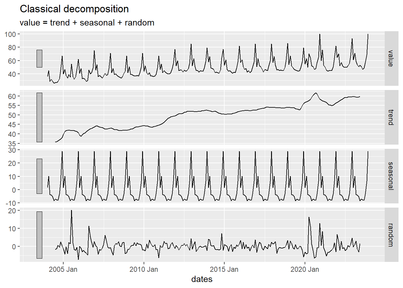
choc_decompose <- chocolate_month_ts |>
    model(feasts::classical_decomposition(value,
        type = "mult"))  |>
    components()

autoplot(choc_decompose)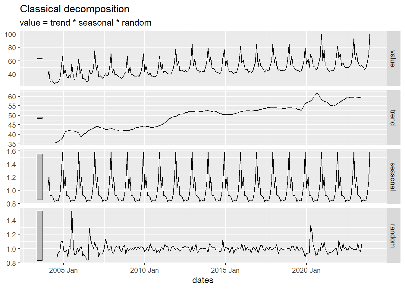

Here are the values of the acf for the chocolate search data:

acf(chocolate_month_ts$value, plot=FALSE, type = "correlation", lag.max = 25)


Autocorrelations of series 'chocolate_month_ts$value', by lag

     0      1      2      3      4      5      6      7      8      9     10 
 1.000  0.522  0.440  0.159  0.041 -0.018 -0.081 -0.024  0.020  0.121  0.386 
    11     12     13     14     15     16     17     18     19     20     21 
 0.425  0.814  0.426  0.357  0.103 -0.001 -0.051 -0.114 -0.057 -0.003  0.104 
    22     23     24     25 
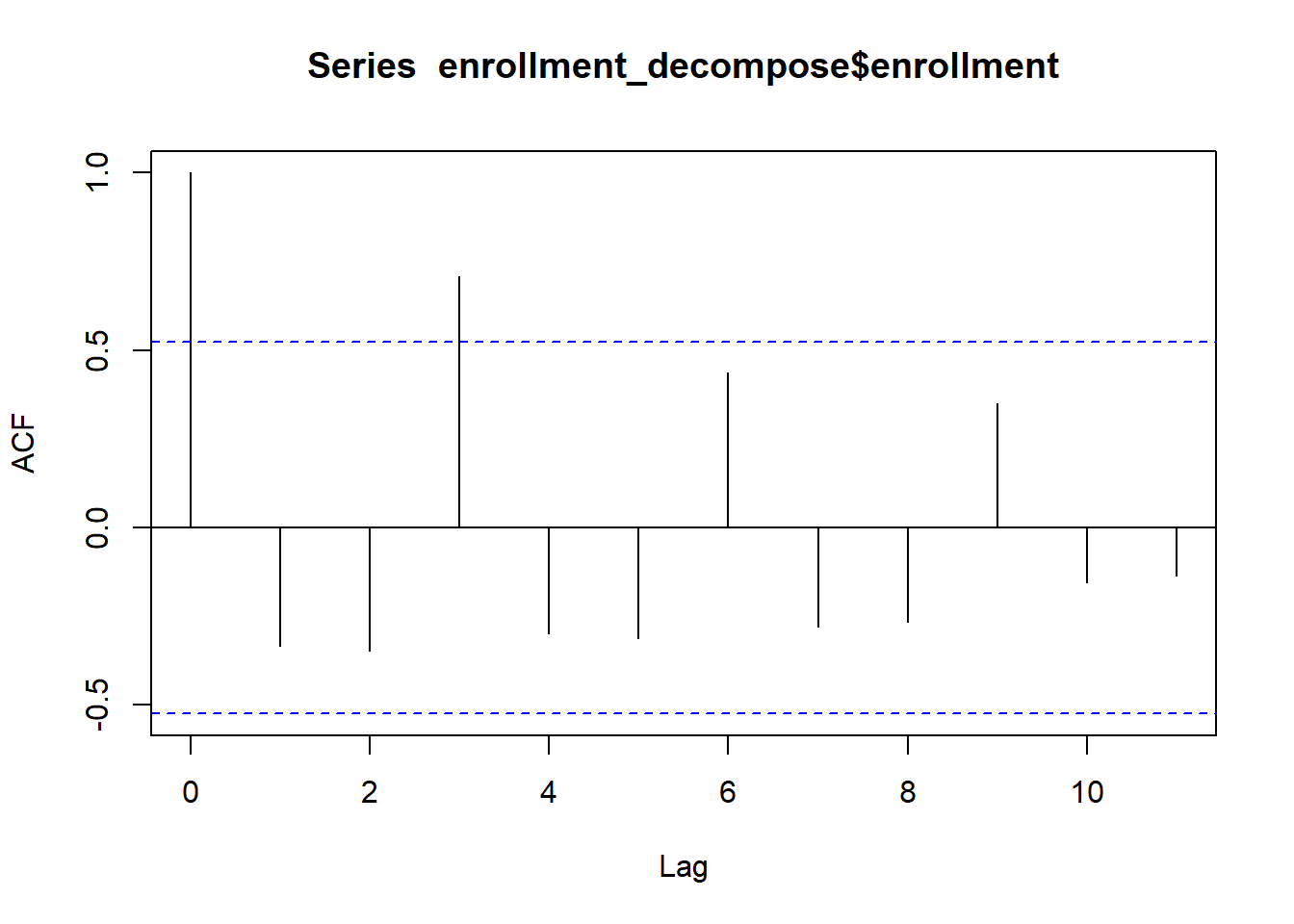
 0.358  0.398  0.768  0.389

Here is the associated correlogram:

acf(chocolate_month_ts$value, plot=TRUE, type = "correlation", lag.max = 25)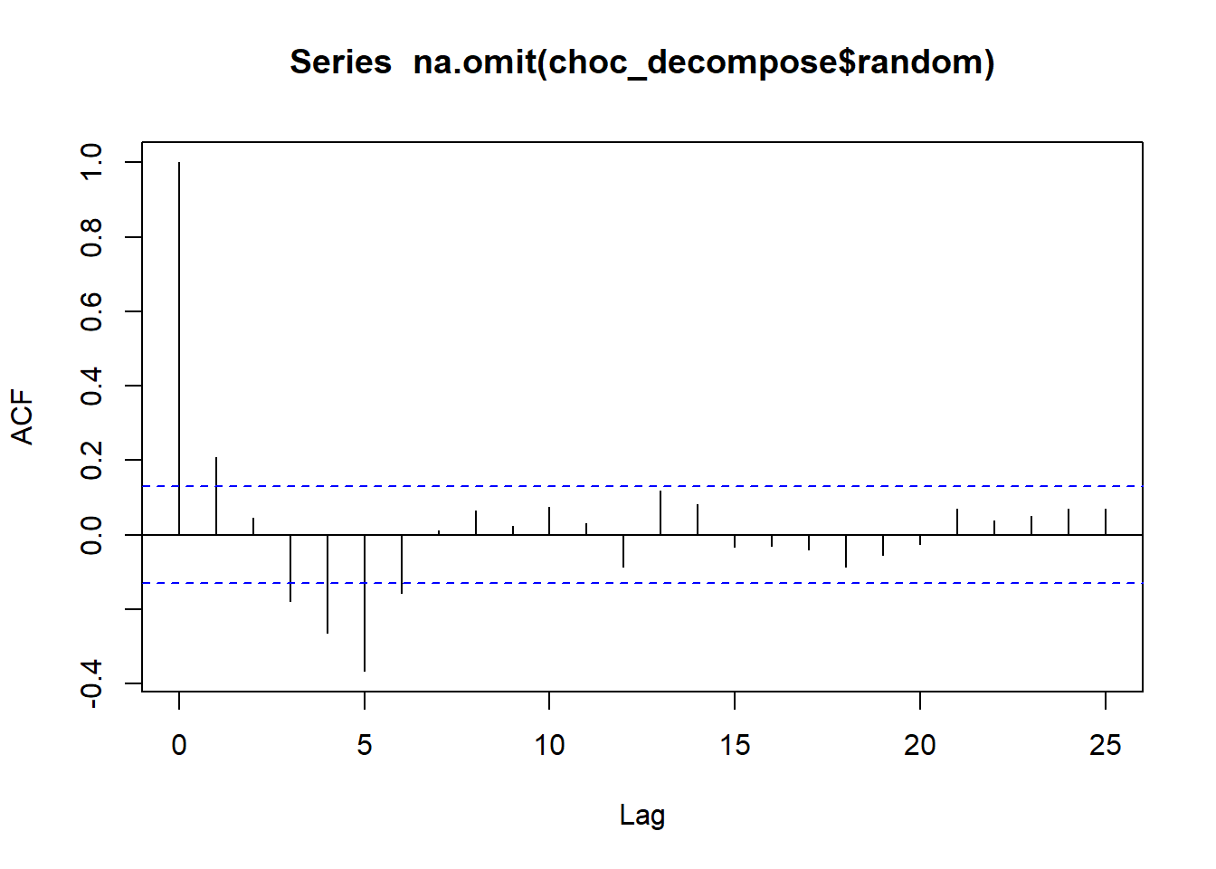

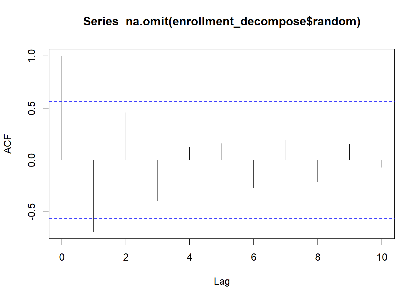
Check Your Understanding

What does the information displayed in this correlogram suggest?

If we consider only the random component of this time series, the correlogram is:

acf(choc_decompose$random |> na.omit(), plot=TRUE, type = "correlation", lag.max = 25)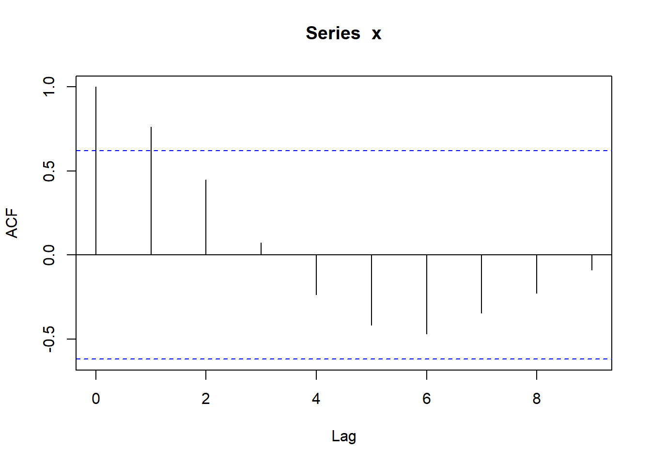

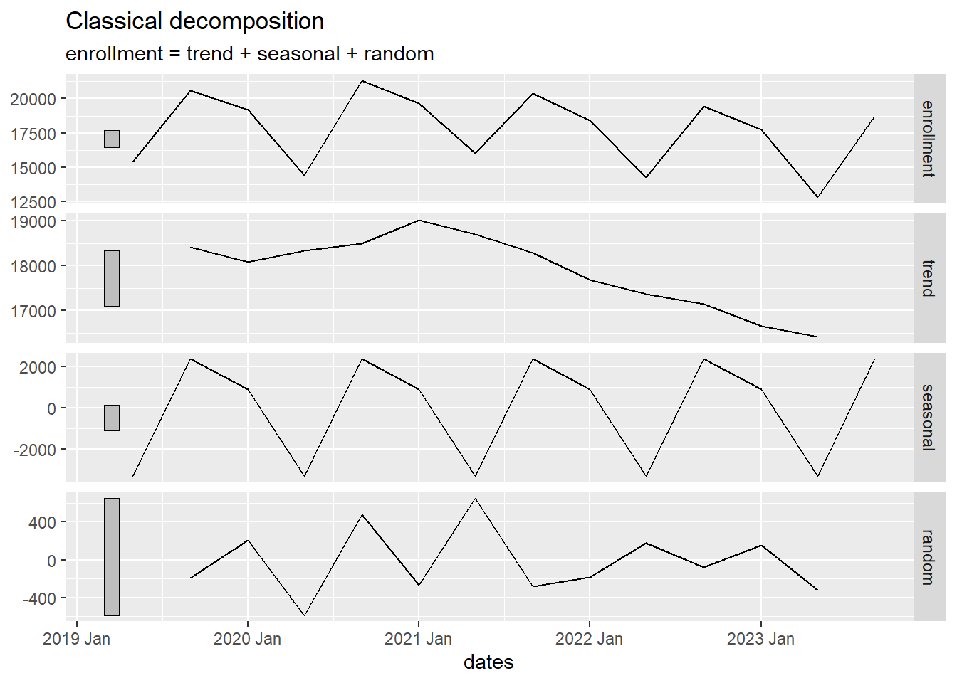
Check Your Understanding

What do the spikes in the correlogram tell us about this time series?
Is there evidence of autocorrelation in the data after removing the trend and seasonal variation?
What would happen to the correlogram of the random component if we used an additive decomposition?

Statistical vs Practical Significance

An estimate for the lag k autocorrelation can be statistically significant, but practically insignificant. The percentage of variation in \(x_t\) explained by \(x_{t+k}\) equals \(r_k^2\). In the example above, \(r_3\approx r_4\approx r_5 \approx 0.2\), which mean that each of the lagged variables estimates explain around 4% of the variation of the chocolate series at their respective lag values. All the estimates are statistically significant, but we should put a lot of practical weight in their significance.

Small Group Activity: BYU-Idaho On-Campus Enrollment (25 min)

The official number of on-campus BYU-Idaho students each semester is given in the file byui_enrollment.csv.

Check Your Understanding

Do the following:

Create a tsibble with the BYU-Idaho enrollment data. (Hint: There are three semesters in a year, so treat the enrollments as observations taken every four months in January, May, and September.)
Plot the decomposition of this time series.
Describe the trend.
Describe the seasonal component.
Is there evidence of seasonal variation? If so, propose an explanation for the seasonal variation.
Create the correlogram for these data.
- What do you observe?
- Does the correlogram support the statement you made about the seasonal component?
Is there evidence of autocorrelation in the data after removing the trend and seasonal variation?

Homework Preview (5 min)

Review upcoming homework assignment
Clarify questions

Homework

Download Homework

homework_2_3.qmd

Correlograms

BYU-Idaho Enrollment