pacman::p_load(
  tidyverse,  # ggplot, mutate(), cleaning...
  tsibble,    # as_tsibble()
  fable,      # model(...), forecast(), tidy(), glance()...
  feasts,     # ACF(), PACF()
  ggtime,     # autoplot() for tsibbles
  patchwork,  # + and / for ggplots
  rio         # import()
)Moving Average (MA) Models
Chapter 6: Lesson 1
Learning Outcomes
Characterize the properties of moving average (MA) models
- Define a moving average (MA) process
- Write an MA(q) model in terms of the backward shift operator
- State the mean and variance of an MA(q) process
- Explain the autocorrelation function of an MA(q) process
- Define an invertible MA process
Fit time series models to data and interpret fitted parameters
- Determine an appropriate MA(q) model to fit to a time series based on the ACF plot
- Fit an MA(q) model to data in R using the arima() function
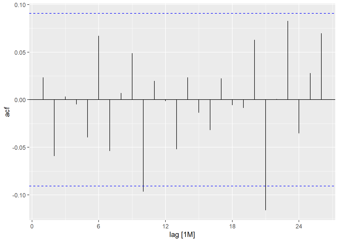
- Assess model fit by examining residual diagnostic plots
- Interpret the fitted MA coefficients
Preparation
- Read Sections 6.1-6.4
Learning Journal Exchange (10 min)
Review another student’s journal
What would you add to your learning journal after reading another student’s?
What would you recommend the other student add to their learning journal?
Sign the Learning Journal review sheet for your peer
Packages
Class Activity: Introduction to Moving Average (MA) Models (15 min)
Stationary Processes
In previous chapters, we have explored how to identify and remove the trend and seasonal components of a time series. After the trend and seasonal component have been properly removed, the residual should be stationary. However, these residual components may still contain autocorrelation.
In this chapter, we will explore stationary models that are appropriate when there are no obvious trends or seasonal elements. Combining the fitted stationary model with the estimated trend and seasonal components can improve our ability to make forecasts. We will build on the autoregressive (AR) models we learned in Chapter 4.
Strictly Stationary Series
First, we define a strictly stationary series.
If a time series is strictly stationary, then its mean and variance are constant in time. Hence, the autocovariance \(cov(x_t, x_s)\) depends only on the lag, \(k = | t - s |\). We can therefore denote the covariance function as \(\gamma(k) = cov(x_t, x_{t+k})\).
Note: It is possible that a series could have a constant mean and variance in time and the autocovariance depends only on the lag, but the series is not strictly stationary. This is called second-order stationary.
We will focus on the second-order properties of the time series, even though all the series we will explore in this chapter are strictly stationary.
Note: if a white noise process is Gaussian, the stochastic process is completely determined by the mean and covariance structure. This is similar to how a (univariate or multivariate) normal distribution is completely specified by the mean and variance-covariance matrix.
The concept of stationarity is a property of time series models. When we use certain models, we are assuming stationarity. Before we apply these models, it is important to check for stationarity in the time series. In other words, we check to see if there is evidence of a trend or seasonality and if so, we remove these components. We can use methods such as decomposition, Holt-Winters, or regression to remove the trend and seasonality. Hence, it is typically reasonable to consider the residual series as a stationary series. Typically the models in this chapter are applied to the residual series from a regression or similar analysis.
Moving Average (MA) Models
Recall in Chapter 4, Lesson 3, we learned the definition of an AR model:
The \(AR(p)\) model can be expressed in terms of the backward shift operator: \[ \left( 1 - \alpha_1 \mathbf{B} - \alpha_2 \mathbf{B}^2 - \cdots - \alpha_p \mathbf{B}^p \right) x_t = w_t \]
Now, we consider a different, but related model, the moving average (MA) model
We now define an invertible \(MA\) process.
Example of an Invertible MA Process
Recall that \[ (1-x)(1 + x + x^2 + x^3 + \cdots) = 1 \]
or,
\[ (1-x)^{-1} = (1 + x + x^2 + x^3 + \cdots) \] if \(|x|<1\).
Now, note that the \(MA\) process
\[ x_t = \left( 1 - \beta \mathbf{B} \right) w_t \]
can be written as:
\[\begin{align*} \left( 1 - \beta \mathbf{B} \right)^{-1} x_t &= w_t \\ \left( 1 + \beta \mathbf{B} + \beta^2 \mathbf{B}^2 + \beta^3 \mathbf{B}^3 + \cdots \right) x_t &= w_t \\ x_t + \beta x_{t-1} + \beta^2 x_{t-2} + \beta^3 x_{t-3} + \cdots &= w_t \\ x_t &= \left( -\beta x_{t-1} - \beta^2 x_{t-2} - \beta^3 x_{t-3} - \cdots \right) + w_t \end{align*}\]
assuming that \(|\beta|<1\). Note that this series will not converge unless \(|\beta|<1\).
We have just shown that the \(MA\) process \[ x_t = \left( 1 - \beta \mathbf{B} \right) w_t \] is invertible.
Does this remind you of the test for the stationarity of an \(AR(p)\) model?
Note that the autocovariance function (acvf) will identify a unique \(MA(q)\) process only if the process is invertible. Fortunately, the algorithm R uses to estimate an \(MA(q)\) process always leads to an invertible model.
Class Activity: Simulating an \(MA(q)\) Model (5 min)
The textbook gives a simulation of an \(MA(3)\) process:
\[ x_t = w_t + \beta_1 w_{t-1} + \beta_2 w_{t-2} + \beta_3 w_{t-3} \]
where \(\beta_1 = 0.7\), \(\beta_1 = 0.5\), and \(\beta_3 = 0.2\). This shiny app allows you to simulate from this process.
Class Activity: Identifying AR and MA Models from the ACF and PACF (5 min)
AR Process
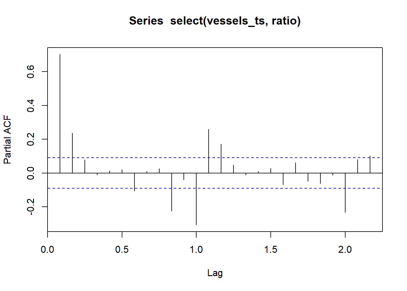
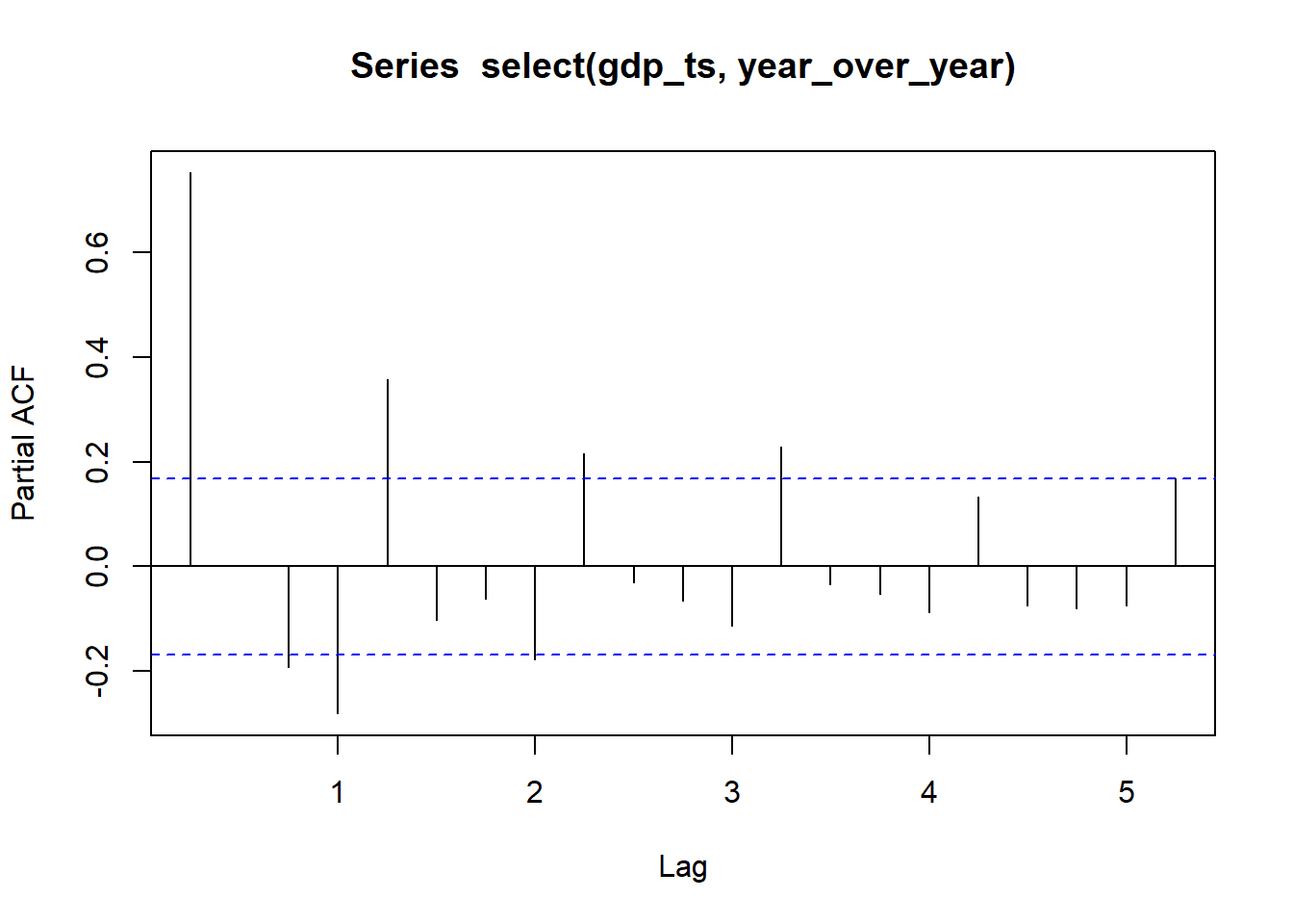
Recall that on page 81, the textbook states that in general, the partial autocorrelation at lag \(k\) is the \(k^{th}\) coefficient of a fitted \(AR(k)\) model. This implies that if the underlying process is \(AR(p)\), then all the coefficients \(\alpha_k\) will equal 0 whenever \(k>p\). So, an \(AR(p)\) process will result in partial correlations that are zero after lag \(p\). So, we can look at the correlogram of partial autocorrelations to determine the order of an appropriate \(AR\) process to model a time series.
MA Process
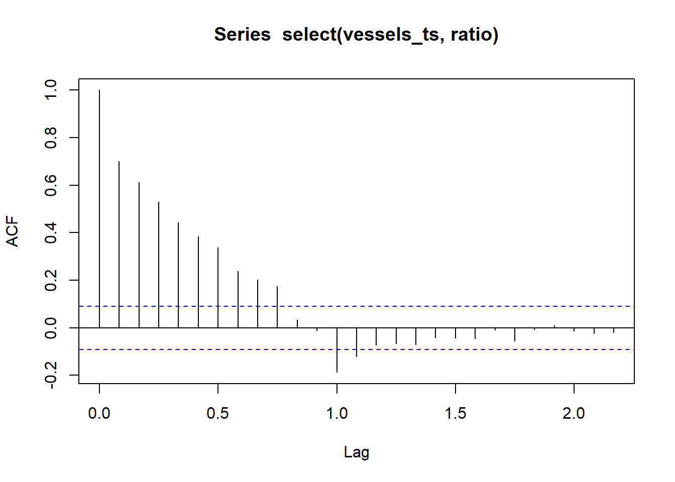
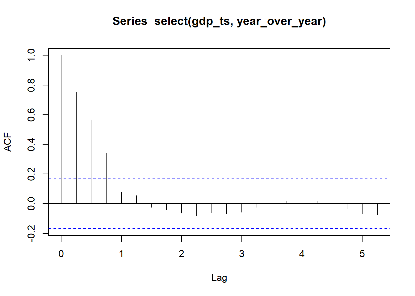
Similarly, for an \(MA(q)\) process, the coefficients \(\beta_k\) will equal 0 whenever \(k > q\). Hence, an \(MA(q)\) process will demonstrate autocorrelations that are 0 after lag \(q\). So, considering the correlogram of autocorrelations, we can assess if an \(MA(q)\) model would be appropriate.
Bless their hearts, the textbook authors give a bad example in Section 6.4.2. They even state that it is “not a realistic realisation.” MA processes naturally arise in ratios of observed data. Multi-period asset returns (i.e. ratios of some previous term’s value) tend to follow an MA process.
For example, if there are 252 trading days in a year, then the daily series of year-over-year returns (this year’s value divided by last year’s value) follows an \(MA(252-1)\) process. If we are comparing values observed to those from one week ago, we would have an \(MA(7-1)\) process.
Comparison
Class Activity: Fitting an \(MA(q)\) Model to GDP Year-Over-Year Ratios (5 min)
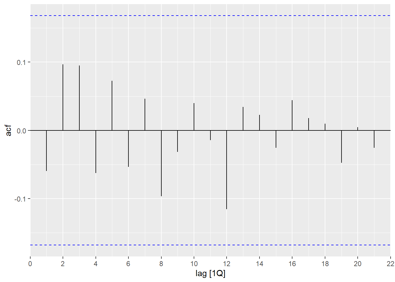
To fit an \(MA(q)\) model, we look at the acf to determine if it cuts off after \(q\) lags.
Show the code
# gdp_ts <- rio::import("https://byuistats.github.io/timeseries/data/gdp_fred.csv") |>
gdp_ts <- rio::import("data/gdp_fred.csv") |>
  mutate(year_over_year = gdp_millions / lag(gdp_millions, 4)) |>
  mutate(quarter = yearquarter(mdy(quarter))) |>
  filter(quarter >= yearquarter(my("Jan 1990")) & quarter < yearquarter(my("Jan 2025"))) |>
  na.omit() |>
  mutate(t = 1:n()) |>
  mutate(std_t = (t - mean(t)) / sd(t)) |>
  as_tsibble(index = quarter)

gdp_ts |>
  autoplot(.vars = gdp_millions) +
    labs(
      x = "Quarter",
      y = "GDP (Millions of $US)",
      title = "U.S. Gross Domestic Product (GDP) in Millions of Dollars"
    ) +
    theme_minimal() +
    theme(plot.title = element_text(hjust = 0.5))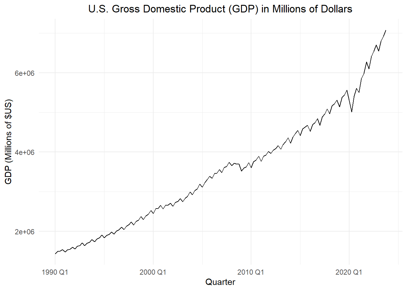
Show the code
gdp_ts |>
  autoplot(.vars = year_over_year) +
  stat_smooth(method = "lm",
              formula = y ~ x,
              geom = "smooth",
              se = FALSE,
              color = "#E69F00",
              linetype = "dotted") +
    labs(
      x = "Quarter",
      y = "Ratio",
      title = "Year-Over-Year Change in U.S. GDP"
    ) +
    theme_minimal() +
    theme(plot.title = element_text(hjust = 0.5))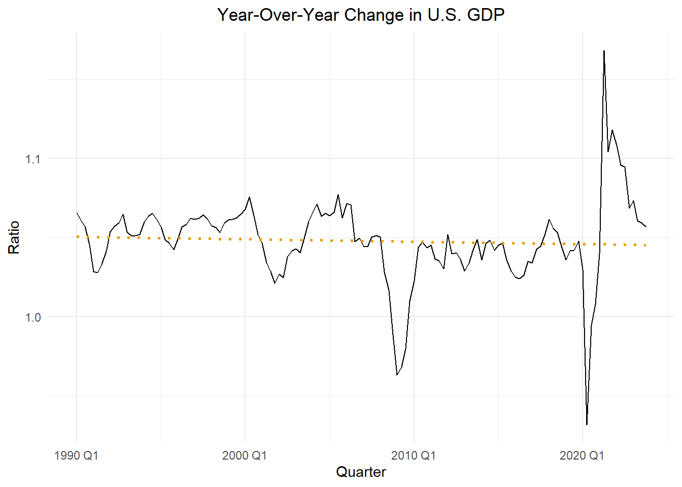
Show the code
gdp_ts |>
  select(year_over_year) |>
  acf()
Show the code
gdp_ts |>
  select(year_over_year) |>
  pacf()
Small-Group Activity: Fitting an \(MA(q)\) Model to the Trade Data (15 min)
Vessels Cleared in Foreign Trade for United States
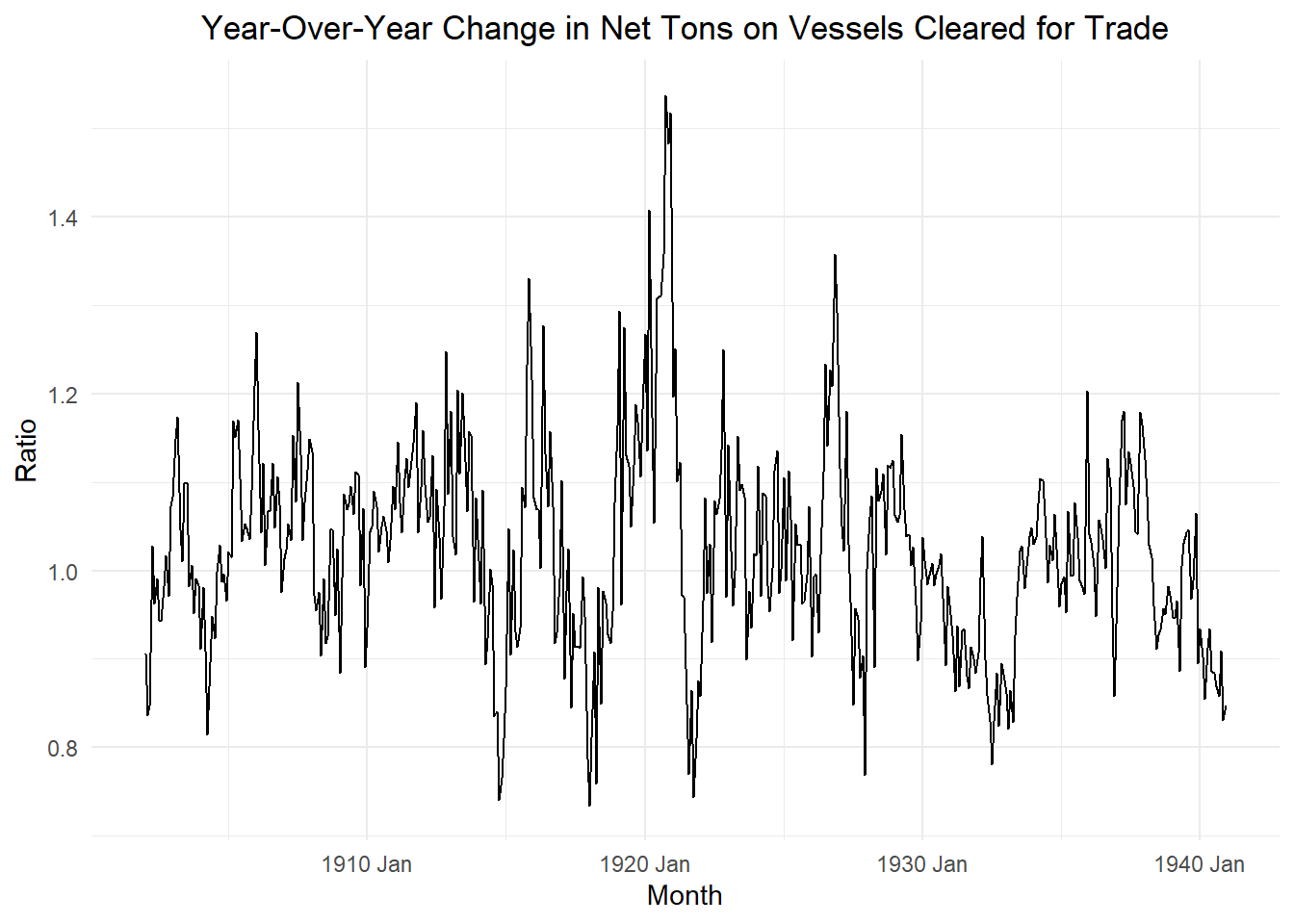
In the homework for Chapter 1 Lesson 5, you explored data on the thousands of net tons cleared in foreign trade for the United States each month from January 1902 to December 1940. The code below computes the year-over-year change in the amount of cargo cleared for trade. This is stored in the variable ratio.
Show the code
vessels_ts <- rio::import("https://byuistats.github.io/timeseries/data/Vessels_Trade_US.csv") |>
  # filter(-comments) |>
  mutate(
    date = yearmonth(dmy(date)),
    ratio = vessels / lag(vessels, 12)
  ) |>
  na.omit() |>
  as_tsibble(index = date)

vessels_ts |>
  autoplot(.vars = ratio) +
    labs(
      x = "Month",
      y = "Ratio",
      title = "Year-Over-Year Change in Net Tons on Vessels Cleared for Trade"
    ) +
    theme_minimal() +
    theme(plot.title = element_text(hjust = 0.5))
Homework Preview (5 min)
- Review upcoming homework assignment
- Clarify questions
MA(q) process in terms of the backward shift operator
Class Activity: Fitting an MA(q) Model to GDP Year-Over-Year Ratios
Small-Group Activity: Fitting an MA(q) Model to the Trade Data