Course Introduction

Chapter 1: Lesson 1

Learning Outcomes

Introduce the course structure and syllabus

Get to know each other
Describe key concepts in time series analysis
Explore an example time series interactively

Introduction to the course structure and Canvas (30 min)

Introduction of teacher(s)
Introduction of students
Syllabus
Software: R and RStudio
Textbook
- Cowpertwait, P. S. P., & Metcalfe, A. V. (2009). Introductory Time Series with R. Springer. ISBN 978-0-387-88697-8; e-ISBN 978-0-387-88698-5; DOI 10.1007/978-0-387-88698-5.
Supplement to the Textbook
- Modern R code
- Time Series (TS) Notebook for in-class activities
Lesson cadence
- Read assigned section(s) from the textbook
  - Assigned sections listed in the TS notebook
- Reading Journals
  - Record your learning
  - Include all of the following from the assigned reading: vocabulary terms, nomenclature, models, important concepts, and your questions
  - Review another student’s learning journal at the beginning of class
- In-class Activities
- Homework
Assessment Structure
- Daily Homework, Multi-week Projects, Three Exams
Grading Categories
- Reading Journal (10%)
- Homework (40%)
- Projects (25%)
- Exams (25%)
Grades: 93% = A
Calendar
Team structure for class activities
- Random assignment, frequent changes, partner with each student in the class
- We are all in this together

Class Activity: Google Trends (Searches for “Chocolate”) (10 min)

Google Trends allows you to download a time series showing the proportional number of searches for a given term. The month with the highest number of searches has a value of 100. The values for the other months are given as a percentage of the peak month’s value. The following table illustrates the data, as given by Google Trends.

Installing package into 'C:/Users/DELL/AppData/Local/R/win-library/4.5'
(as 'lib' is unspecified)

also installing the dependencies 'fontBitstreamVera', 'fontLiberation', 'fontquiver', 'gdtools', 'ggiraph', 'ggridges', 'labelled', 'ggformula', 'mosaicData', 'mosaicCore'

Warning: unable to access index for repository http://www.stats.ox.ac.uk/pub/RWin/bin/windows/contrib/4.5:
  cannot open URL 'http://www.stats.ox.ac.uk/pub/RWin/bin/windows/contrib/4.5/PACKAGES'

package 'fontBitstreamVera' successfully unpacked and MD5 sums checked
package 'fontLiberation' successfully unpacked and MD5 sums checked
package 'fontquiver' successfully unpacked and MD5 sums checked
package 'gdtools' successfully unpacked and MD5 sums checked
package 'ggiraph' successfully unpacked and MD5 sums checked
package 'ggridges' successfully unpacked and MD5 sums checked
package 'labelled' successfully unpacked and MD5 sums checked
package 'ggformula' successfully unpacked and MD5 sums checked
package 'mosaicData' successfully unpacked and MD5 sums checked
package 'mosaicCore' successfully unpacked and MD5 sums checked
package 'mosaic' successfully unpacked and MD5 sums checked

The downloaded binary packages are in
    C:\Users\DELL\AppData\Local\Temp\Rtmp4ODnDW\downloaded_packages


mosaic installed

                                     
 Category: All categories            
                                     
 Month     chocolate: (United States)
 2004-01                           36
 2004-02                           45
 2004-03                           29
 2004-04                           32
 2004-05                           29
 2004-06                           26
 2004-07                           27
 2004-08                           27
 2004-09                           29
 2004-10                           33
 2004-11                           46
 2004-12                           67
 2005-01                           40
    ⋮                               ⋮
 2023-10                           57
 2023-11                           69
 2023-12                          100

The cleaned version of the data used for this demonstration are available in the file chocolate.csv. We can read this directly into a data frame using the command

chocolate_month <- rio::import("https://byuistats.github.io/timeseries/data/chocolate.csv")

In Lesson 3, we will practice converting data like this into a time series (tsibble) object.

Show the code

if (!require("pacman")) install.packages("pacman")
pacman::p_load("tsibble", "fable",
               "feasts", "tsibbledata",
               "fable.prophet", "tidyverse",
               "patchwork", "rio")

# read in the data from a csv and make the tsibble
# change the line below to include your file path
chocolate_month <- rio::import("https://byuistats.github.io/timeseries/data/chocolate.csv")
start_date <- lubridate::ymd("2004-01-01")
date_seq <- seq(start_date,
                start_date + months(nrow(chocolate_month)-1),
                by = "1 months")
chocolate_tibble <- tibble(
  dates = date_seq,
  year = lubridate::year(date_seq),
  month = lubridate::month(date_seq),
  value = dplyr::pull(chocolate_month, chocolate)
)
chocolate_month_ts <- chocolate_tibble |>
  mutate(index = tsibble::yearmonth(dates)) |>
  as_tsibble(index = index)

chocolate_month_ts |> head()

# A tsibble: 6 x 5 [1M]
  dates       year month value    index
  <date>     <dbl> <dbl> <int>    <mth>
1 2004-01-01  2004     1    36 2004 Jan
2 2004-02-01  2004     2    45 2004 Feb
3 2004-03-01  2004     3    29 2004 Mar
4 2004-04-01  2004     4    32 2004 Apr
5 2004-05-01  2004     5    29 2004 May
6 2004-06-01  2004     6    26 2004 Jun

For now, we will use the tsibble object (which in this case is called chocolate_month_ts) to explore the time series. Here is a plot of the time series representing the proportional frequency of searches for the term “chocolate.”

Show the code

autoplot(chocolate_month_ts, .vars = value) +
  labs(
    x = "Month",
    y = "Searches",
    title = "Relative Number of Google Searches for 'Chocolate'"
  ) +
  theme(plot.title = element_text(hjust = 0.5))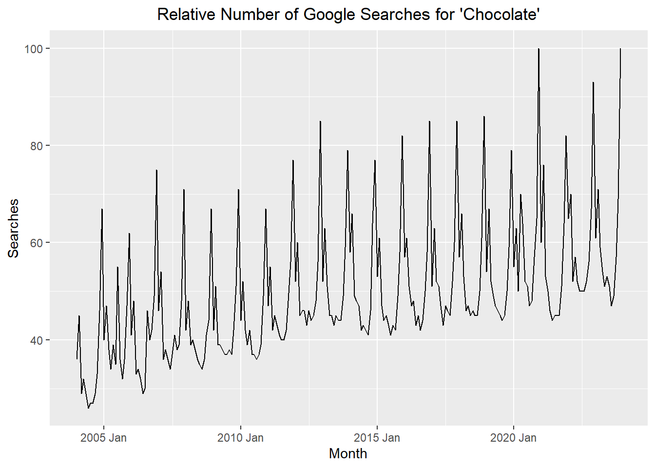

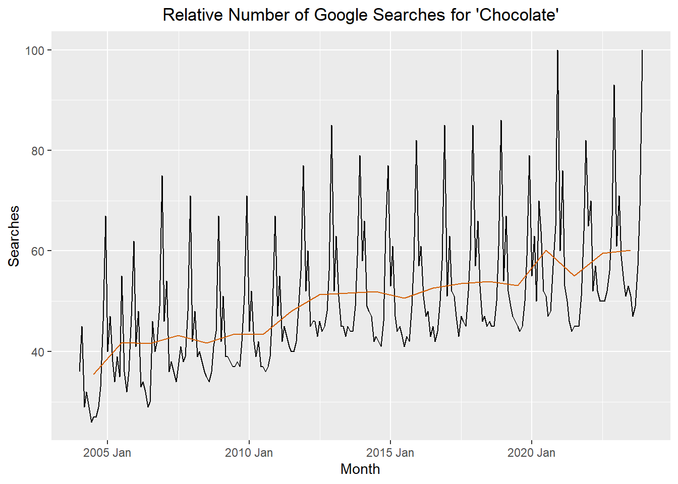
Warning: `autoplot.tbl_ts()` was deprecated in fabletools 0.6.0.
ℹ Please use `ggtime::autoplot.tbl_ts()` instead.
ℹ Graphics functions have been moved to the {ggtime} package. Please use
  `library(ggtime)` instead.

Check Your Understanding

What do you notice about this plot?

The red line represents the mean for each year. The point for this line was positioned to align with July of the year.

Check Your Understanding

What do you observe about the number of searches for “chocolate” each month?
What might be causing this trend?

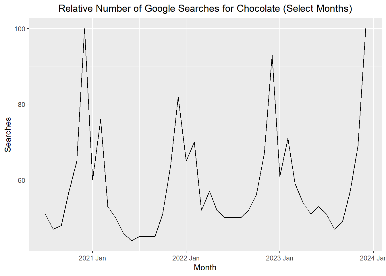
Consider the data for the last few years:

Check Your Understanding

Which month tends to have the greatest number of Google searches for “chocolate”?
Which month has the second greatest number of Google searches for “chocolate”?
When do the fewest number of Google searches for “chocolate” occur?
How can you explain these observations?

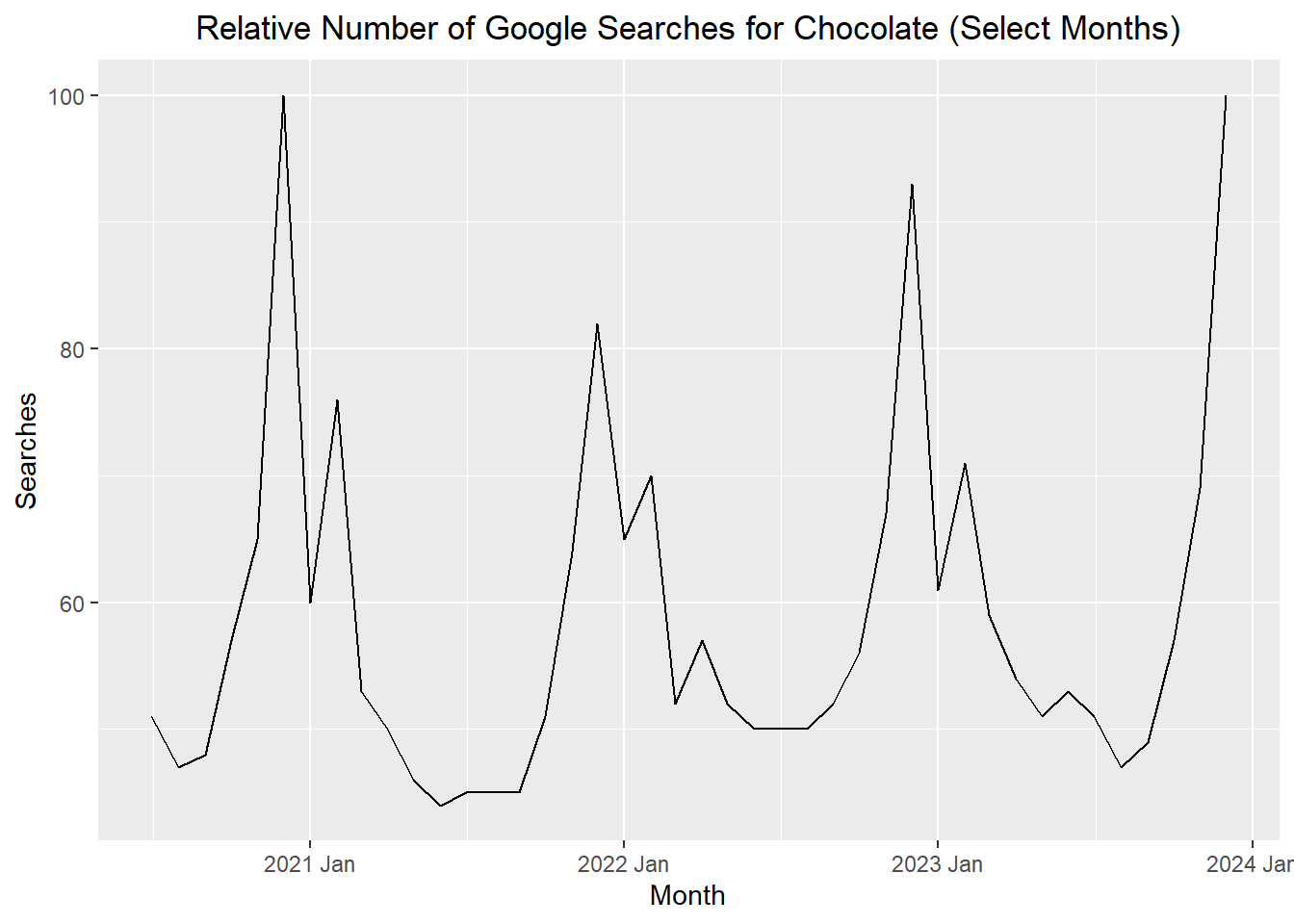
Autocorrelation is a fancy word that means that sequential values in a sequence of data are related in some way.

Consider searches in successive months. Are they independent?

Check Your Understanding

Think about what you know about the reported number of searches in December compared to the following February. The reported number of searches for “chocolate” in December 2022 is 93. Does it make sense that the reported number of searches in February 2023 is 71 ? Given the value from December, is the value in the following February independent and completely random?
The value reported by Google for June 2023 is 53. Based on what you have observed in the data, do you think the value for July 2023 will be close to or far from this value? Justify your answer.

Discuss these vocabulary terms in the context of the Google Trends (“Chocolate”) example: - Time series - Sampling interval - Autocorrelation (or serial dependence) - Trend - Seasonal variation - Cycle

Class Activity: S&P 500 (10 min)

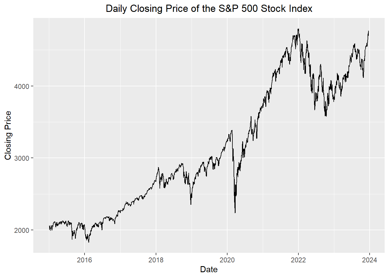
The time series plot below illustrates the daily closing prices of the standard and Poor’s 500 stock index (S&P 500).

The red line represents the mean for each year. The point for this line was positioned to align with July of the year.

Check Your Understanding

What do you observe about the value of the S&P 500 over time?
What might be causing this trend?

Check Your Understanding

Are there regularly-occurring seasonal trends in the data?
Are there some random (stochastic) business cycles observable in the data?
How can you explain these observations?

Check Your Understanding

Consider closing prices in successive days. Are they independent?
Why would there be autocorrelation in the data?

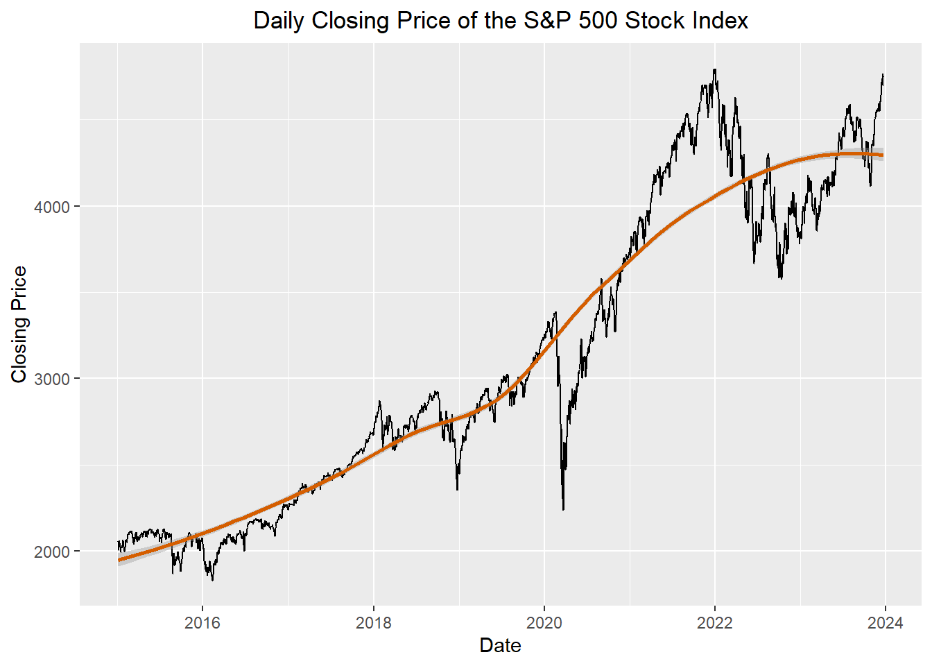
Discuss these vocabulary terms in the context of the S&P 500 example:

Time series
Sampling interval
Autocorrelation (or serial dependence)
Trend
Seasonal variation
Cycle
Deterministic vs. Stochastic

Recap (5 min)

What is time series data?
- Define “time series” (e.g. observations collected sequentially over time)
Examples of time series data
Why ordinary regression fails – correlated error terms
Examples of time series from different domains:
- Daily credit card balance
- Daily closing stock prices
- Monthly sales figures
- Yearly global temperature measurements
- Secondly wave heights in an ocean buoy
- Weekly unemployment rates
- Quarterly GDP estimates
Importance of context and subject matter knowledge
Role of models (explanation, prediction, simulation)
Are there any questions on the course or time series data?

Homework Preview (5 min)

Review upcoming homework assignment
Clarify questions

Homework

Download Assignment

homework_1_1.qmd

Preparation for the next class meeting

Update R and RStudio
Access
- Canvas course
- Time Series Notebook (Quarto file)
Purchase the textbook
Read sections 1.1-1.4 in the textbook
Obtain a Learning Journal
Prepare to share your Learning Journal with another student in the next class meeting