Averages for Time Series

Chapter 1: Lesson 3

Learning Outcomes

Decompose time series into trends, seasonal variation, and residuals

• Define smoothing
• Compute the centered moving average for a time series
• Estimate the trend component using moving averages

Plot time series data to visualize trends, seasonal patterns, and potential outliers

• Plot the estimated trend of a time series using a moving average
• Make box plots to examine seasonality
• Interpret the trend and seasonal pattern observed in a time series

Preparation

• Read Sections 1.5.1-1.5.3

Learning Journal Exchange (10 min)

• Review another student’s journal
• What would you add to your learning journal after reading your partner’s?
• What would you recommend your partner add to their learning journal?
• Sign the Learning Journal review sheet for your peer

Vocabulary and Nomenclature Matching Activity (10 min)

Check Your Understanding

Working with a partner, match the definitions on the left with the terms on the right.

Nomenclature Matching

8. Discrete observations of a time series, taken at times \(1, 2, \ldots, n\).
9. Number of observations of a time series
10. Lead time
11. The trend as observed at time \(t\)
12. The seasonal effect, as observed at time \(t\)
13. The error term (a sequence of correlated random variables with mean zero), as observed at time \(t\)
14. Centered moving average for obsrvations made monthly
15. Estimate of monthly additive effect
16. Estimate of monthly multiplicative effect

8. \(n\)
9. \(k\)
10. \(m_t\)
11. \(\hat m_t\)
12. \(s_t\)
13. \(\hat s_t = x_t - \hat m_t ~~~~~~~~~~~~~~~~~~~~~~~~~\)
14. \(\hat s_t = \dfrac{x_t}{\hat m_t}\)
15. \(\{x_t\}\)
16. \(z_t\)

where \(\hat m_t = \dfrac{\frac{1}{2}x_{t-6} + x_{t-5} + \cdots + x_{t-1} + x_t + x_{t+1} + \cdot + x_{t+5} + \frac{1}{2} x_{t+6}}{12}\).

Additional Nomenclature Matching

17. Forecast made at time \(t\) for a future value \(k\) time units in the future \(~~~~~~~~~~~~~~~~~~~~~~\)
18. Additive decomposition model
19. Additive decomposition model after taking the logarithm
20. Multiplicative decomposition model
21. Seasonally adjusted mean for the month corresponding to time \(t\)
22. Seasonal adjusted series (additive seasonal effect)
23. Seasonal adjusted series (multiplicative seasonal effect)

17. \(\bar s_t\)
18. \(x_t = m_t + s_t + z_t\)
19. \(x_t = m_t \cdot s_t + z_t\)
20. \(\log(x_t) = m_t + s_t + z_t\)
21. \(x_t - \bar s_t\)
22. \(\frac{x_t}{\bar s_t}\)
23. \(\hat x_{t+k \mid t}\)

Team Activity: Moving Averages (30 min)

Derivation

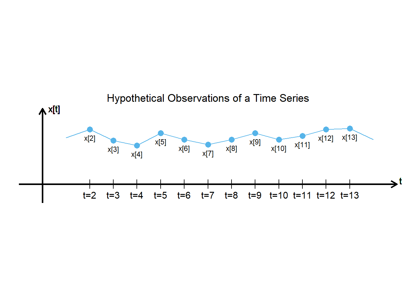
Data representing some value have been collected each month for a few years. This plot represents the first 12 observations in this time series.

Check Your Understanding

• Suppose you wanted to compute the mean of the observations from the first year (\(t = 1\) to \(t=12\).) What is the formula you would use to compute this mean? Write this expression without a summation symbol.
• To what value of \(t\) should this mean be assigned? (If you were to plot this mean on a time plot, where should it go?)

Check Your Understanding

• Suppose you want to compute the mean of one year’s worth of observations, beginning at month \(t=2\). Write the formula you would use to compute this mean without using a summation symbol.
• To what value of \(t\) should this mean be assigned? (If you were to plot this mean on a time plot, where should it go?)

Check Your Understanding

• Note that neither of the two means above are appropriately located on an integer value of \(t\).
• Give the formula that combines the two means above to give one mean that is centered on an integer value of \(t\). Do not include a summation symbol in your formula. (Hint: try averaging the two means.)
• Upon what value of \(t\) is your new mean centered?

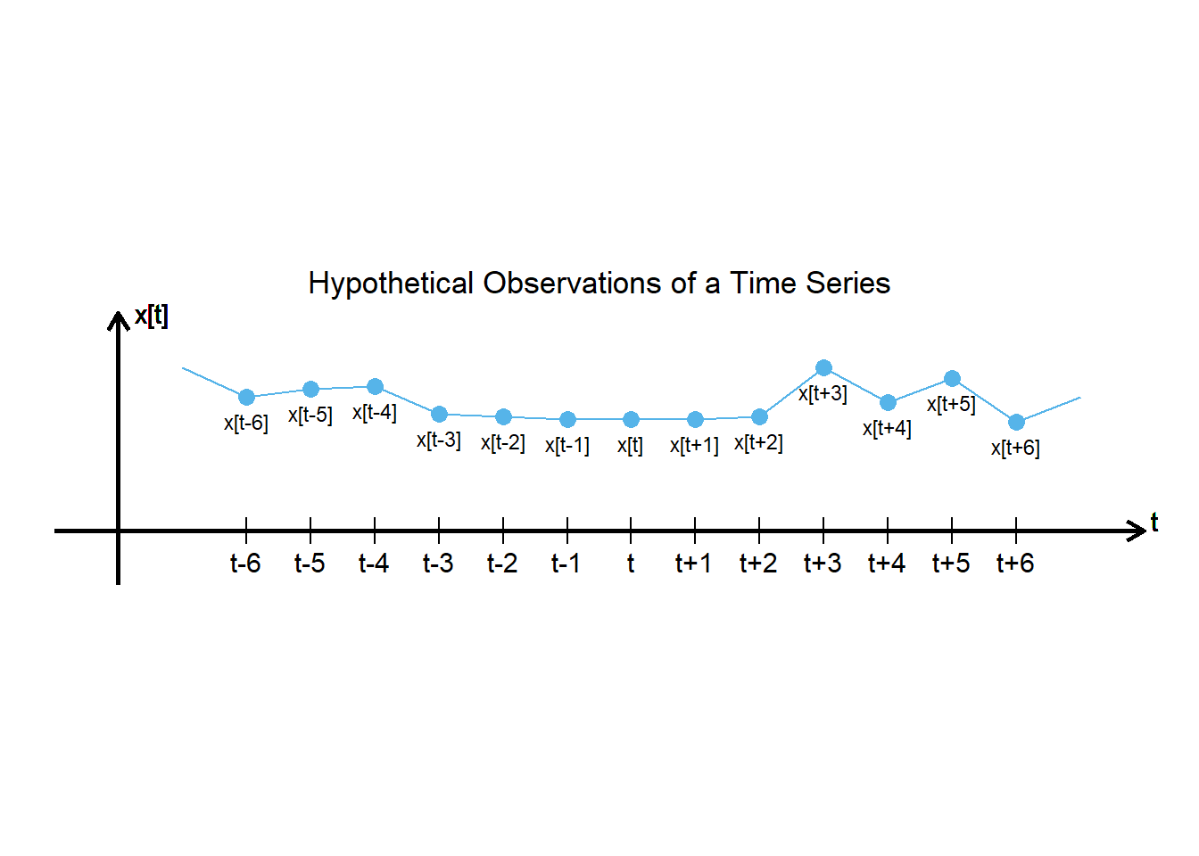
We will now adjust this moving average adjusted so it is centered on any given value of \(t\), not just \(t=7\).

Check Your Understanding

• Consider the values \(x_{t-6}\), \(x_{t-5}\), \(x_{t-4}\), \(x_{t-3}\), \(x_{t-2}\), \(x_{t-1}\), \(x_{t}\), \(x_{t+1}\), \(x_{t+2}\), \(x_{t+3}\), \(x_{t+4}\), and \(x_{t+5}\).
  • Give an expression for the mean of the values.
  • Where will this mean be centered?
• Consider the values \(x_{t-5}\), \(x_{t-4}\), \(x_{t-3}\), \(x_{t-2}\), \(x_{t-1}\), \(x_{t}\), \(x_{t+1}\), \(x_{t+2}\), \(x_{t+3}\), \(x_{t+4}\), \(x_{t+5}\), and \(x_{t+6}\).
  • Give an expression for the mean of the values.
  • Where will this mean be centered?
• We now combine these two means by averaging them.
  • Give an expression for the mean of these two means.
  • Where will this combined mean be centered?

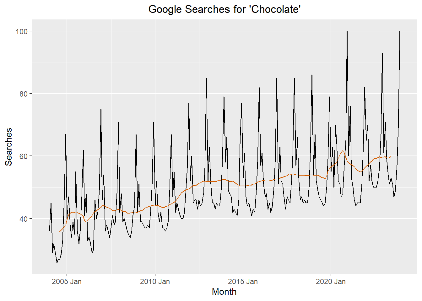
Application: Google Trends Searches for “Chocolate”

Recall the Google Trends data for the term “chocolate” given in the file chocolate.csv.

# load packages
if (!require("pacman")) install.packages("pacman")
pacman::p_load("tsibble", "fable",
               "feasts", "tsibbledata",
               "fable.prophet", "tidyverse",
               "patchwork", "rio")

# read in the data from a csv and make the tsibble
# change the line below to include your file path
chocolate_month <- rio::import("https://byuistats.github.io/timeseries/data/chocolate.csv")
start_date <- lubridate::ymd("2004-01-01")
date_seq <- seq(start_date,
                start_date + months(nrow(chocolate_month)-1),
                by = "1 months")
chocolate_tibble <- tibble(
  dates = date_seq,
  year = lubridate::year(date_seq),
  month = lubridate::month(date_seq),
  value = pull(chocolate_month, chocolate)
)
chocolate_month_ts <- chocolate_tibble |>
  mutate(index = tsibble::yearmonth(dates)) |>
  as_tsibble(index = index)

Check Your Understanding

• Using any tool (except R functions that automate the process) compute the centered moving average for the chocolate data. To help your check yourself, the value of \(\hat m\) in month 7 should be 35.6667.
• Create a plot of your centered moving average. Here are some examples of ways you could display your centered moving average.

Check Your Understanding

• What does the centered moving average reveal about the chocolate search time series?
• Suppose the chocolate data were reported daily. How would you compute the moving average? (Note: there are 365 days in a year.)

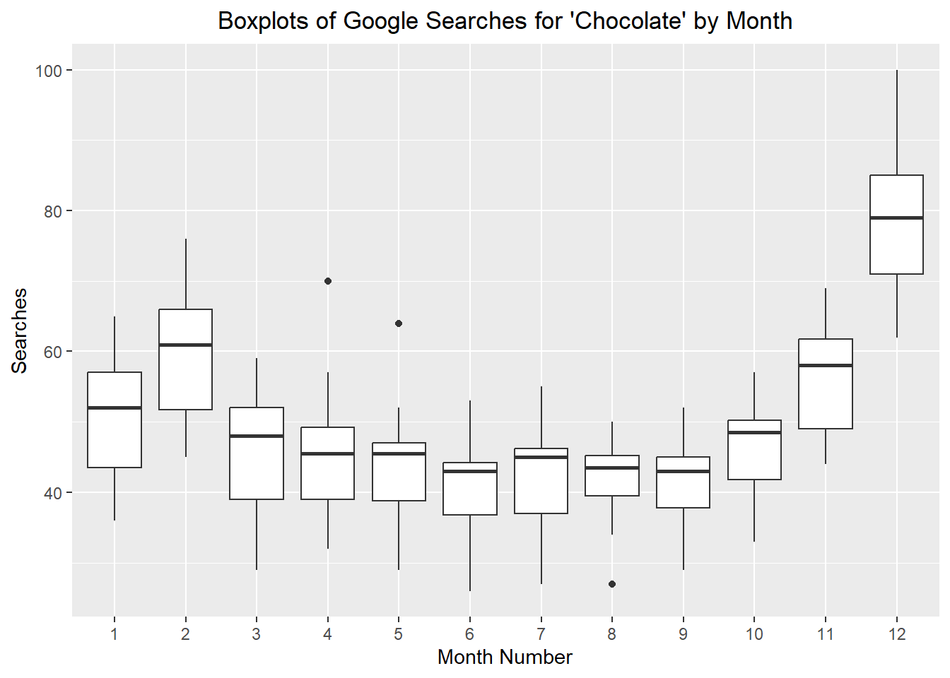
Estimating the Seasonal Effect: Side-by-Side Box Plots by Month (10 min)

To better visualize the effect of seasonal variation, we can make box plots by month.

ggplot(chocolate_month_ts, aes(x = factor(month), y = value)) +
    geom_boxplot() +
  labs(
    x = "Month Number",
    y = "Searches",
    title = "Boxplots of Google Searches for 'Chocolate' by Month"
  ) +
  theme(plot.title = element_text(hjust = 0.5))

Check Your Understanding

• What do you observe?
• Which months tend to have the most searches? Which months tend to have the fewest seraches?
  • Can you provide an explanation for this?

Summary

Check Your Understanding

• What does the centered moving average tell us?
• Why is a centered moving average helpful when there are seasonal effects?
• For the chocolate search data, answer the following questions:
  • How many values of \(t\) were not assigned a value of the centered moving average?
  • Interpret that number in years.
  • Does this number depend on the length of the time series?

Homework Preview (5 min)

• Review upcoming homework assignment
• Clarify questions

Homework

Download Assignment

homework_1_3.qmd

Matching

Check Your Understanding

Matching Solutions

Nomenclature Matching

8. Discrete observations of a time series, taken at times \(1, 2, \ldots, n\).	O. \(\{x_t\}\)
9. Number of observations of a time series	H. \(n\)
10. Lead time	I. \(k\)
11. The trend as observed at time \(t\)	J. \(m_t\)
12. The seasonal effect, as observed at time \(t\)	L. \(s_t\)
13. The error term (a sequence of correlated random variables with mean zero), as observed at time \(t\)	P. \(z_t\)
14. Centered moving average for obsrvations made monthly	K. \(\hat m_t\)
15. Estimate of monthly additive effect	M. \(\hat s_t = x_t - \hat m_t\)
16. Estimate of monthly multiplicative effect	N. \(\hat s_t = \dfrac{x_t}{\hat m_t}\)

Additional Nomenclature Matching

17. Forecast made at time \(t\) for a future value \(k\) time units in the future	W. \(\hat x_{t+k \mid t}\)
18. Additive decomposition model	R. \(x_t = m_t + s_t + z_t\)
19. Additive decomposition model after taking the logarithm	T. \(\log(x_t) = m_t + s_t + z_t\)
20. Multiplicative decomposition model	S. \(x_t = m_t \cdot s_t + z_t\)
21. Seasonally adjusted mean for the month corresponding to time \(t\)	Q. \(\bar s_t\)
22. Seasonal adjusted series (additive seasonal effect)	U. \(x_t - \bar s_t\)
23. Seasonal adjusted series (multiplicative seasonal effect)	V. \(\frac{x_t}{\bar s_t}\)

Team Activity

Solution to Team Activity:

If you stored your centered moving average in a variable called “m_hat” in the “chocolate_month_ts” tsibble, you can generate the superimposed plot with the R command:

chocolate_month_ts <- chocolate_month_ts %>% 
  mutate(
    m_hat = (
          (1/2) * lag(value,6)
          + lag(value,5)
          + lag(value,4)
          + lag(value,3)
          + lag(value,2)
          + lag(value,1)
          + value
          + lead(value,1)
          + lead(value,2)
          + lead(value,3)
          + lead(value,4)
          + lead(value,5)
          + (1/2) * lead(value,6)
        ) / 12
  )

autoplot(chocolate_month_ts, .vars = value) +
  labs(
    x = "Month",
    y = "Searches",
    title = "Google Searches for 'Chocolate'"
  ) +
  geom_line(aes(x = dates, y = m_hat), color = "#D55E00") +
  theme(plot.title = element_text(hjust = 0.5))