pacman::p_load(
  tidyverse,  # ggplot, mutate(), cleaning...
  tsibble,    # as_tsibble()
  fable,      # model(...), forecast(), tidy(), glance()...
  feasts,     # ACF(), PACF()
  ggtime,     # autoplot() for tsibbles
  patchwork,  # + and / for ggplots
  rio         # import()
)Linear Models, Autoregression Errors, and Seasonal Indicator Variables
Chapter 5: Lesson 1
Learning Outcomes
Explain the difference between stochastic and deterministic trends in time series
- Describe deterministic trends as smooth, predictable changes over time
- Define stochastic trends as random, unpredictable fluctuations
- Explain the different treatment of stochastic and deterministic trends when forecasting
Fit linear regression models to time series data
- Define a linear time series model
- Explain why ordinary linear regression systematically underestimates of the standard error of parameter estimates when the error terms are autocorrelated
- Apply generalized least squares GLS in R to estimate linear regression model parameters
- Explain how to estimate the autocorrelation input for the GLS algorithm
- Compare GLS and OLS standard error estimates to evaluate autocorrelation bias
- Identify an appropriate function to model the trend in a given time series
- Represent seasonal factors in a regression model using indicator variables
- Fit a linear model for a simulated time series with linear time trend and \(AR(p)\) error
- Use acf and pacf to test for autocorrelation in the residuals
- Estimate a seasonal indicator model using GLS
- Forecast using a fitted GLS model with seasonal indicator variables
Apply differencing to nonstationary time series
- Transform a non-stationary linear to a stationary process using differencing
- State how to remove a polynomial trend of order \(m\)
Simulate time series
- Simulate a time series with a linear time trend and a \(AR(p)\) error
Preparation
- Read Sections 5.1-5.5
Learning Journal Exchange (10 min)
Review another student’s journal
What would you add to your learning journal after reading another student’s?
What would you recommend the other student add to their learning journal?
Sign the Learning Journal review sheet for your peer
Packages
Small Group Activity: Linear Models (5 min)
Definition of Linear Models
With a partner, practice determining which models are linear and which are non-linear.
Stationarity of Linear Models
The book presents a time series that is modeled as a linear function of time plus white noise: \[ x_t = \alpha_0 + \alpha_1 t + z_t \]
If we difference these values, we get: \[ \begin{align*} \nabla x_t &= x_t - x_{t-1} \\ &= \left[ \alpha_0 + \alpha_1 t + z_t \right] - \left[ \alpha_0 + \alpha_1 (t-1) + z_t \right] \\ &= z_t - z_{t-1} + \alpha_1 \end{align*} \]
Given that the white noise process \(\{ z_t \}\) is stationary, then \(\{ \nabla x_t \}\) is stationary. Differencing is a powerful tool for making a time series stationary.
In Chapter 4 Lesson 2, we established that taking the difference of a non-stationary time series with a stochastic trend can convert it to a stationary time series. Later in the same lesson, we learn that a linear deterministic trend can be removed by taking the first difference. A quadratic deterministic trend can be removed by taking the second differences, and so on.
Note
In general, if there is an \(m^{th}\) degree polynomial trend in a time series, we can remove it by taking \(m\) differences.
Class Activity: Fitting Models (15 min)
Simulation
In Section 5.2.3, the textbook illustrates the time series
\[ x_t = 50 + 3t + z_t \]
where \(\{ z_t \}\) is the \(AR(1)\) process \(z_t = 0.8 z_{t-1} + w_t\) and \(\{ w_t \}\) is a Gaussian white noise process with \(\sigma = 20\). The code below simulates this time series and creates the resulting time plot.
Show the code
set.seed(1)

# Generate data
dat <- tibble(w = rnorm(100, sd = 20)) |>
    mutate(
        Time = 1:n(),
         z = purrr::accumulate2(
            lag(w), w,
            \(acc, nxt, w) 0.8 * acc + w,
            .init = 0)[-1],
          x = 50 + 3 * Time + z
            ) |>
    tsibble::as_tsibble(index = Time)

# Plot data
dat |> autoplot(.var = x) + theme_minimal()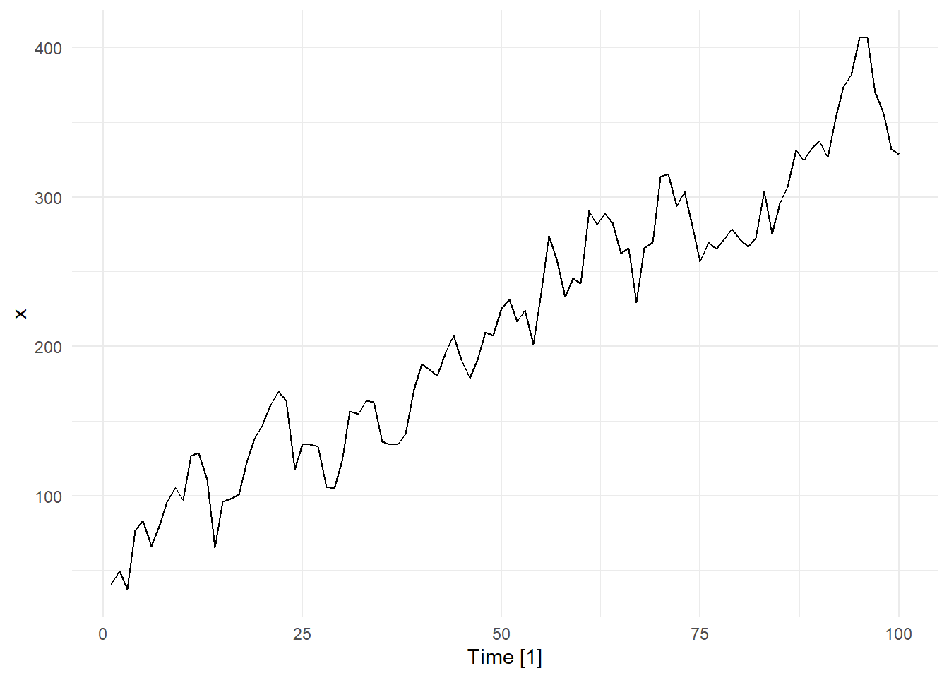
The advantage of simulation is that when we fit a model to the data, we can asses the fit…we know exactly what was simulated.
Model Fitted to the Simulated Data
When applying ordinary least-squares multiple regression, it is common to fit the model by minimizing the sum of squared errors:
\[ \sum r_i^2 = \sum \left( x_t - \left[ \alpha_0 + \alpha_1 u_{1,t} + \alpha_2 u_{2,t} + \ldots + \alpha_m u_{m,t} \right] \right)^2 \]
We assume that the simulated time series above follows the model
\[ x_t = \alpha_0 + \alpha_1 t + z_t \]
In R, we typically accomplish this using the lm function.
dat_lm <- dat |>
  model(lm = TSLM(x ~ Time))
params <- tidy(dat_lm) |> pull(estimate)
stderr <- tidy(dat_lm) |> pull(std.error)
This gives the fitted equation
\[ \hat x_t = 58.551 + 3.063 t \]
The standard errors of these estimated parameters tend to be underestimated by the ordinary least squares method. To illustrate this, a simulation of n = 1000 realizations of the time series above was conducted.
The parameter estimates and their standard errors are summarized in the table below. The “Computed SE” is the standard error reported by the lm function in R. The “Simulated SE” is the standard deviation of the parameter estimated obtained in the 1000 simulated realizations of this time series.
Show the code
# This code simulates the data for this example
# n <- 1000
#
# parameter_est <- data.frame(alpha0 = numeric(), alpha1 = numeric())
# for(count in 1:n) {
#   dat <- tibble(w = rnorm(100, sd = 20)) |>
#       mutate(
#           Time = 1:n(),
#            z = purrr::accumulate2(
#               lag(w), w,
#               \(acc, nxt, w) 0.8 * acc + w,
#               .init = 0)[-1],
#             x = 50 + 3 * Time + z
#               ) |>
#       tsibble::as_tsibble(index = Time)
#
#   dat_lm <- dat |>
#   model(lm = TSLM(x ~ Time))
#
#   parameters <- tidy(dat_lm) |> pull(estimate)
#   parameter_est <- parameter_est |>
#     bind_rows(data.frame(alpha0 = parameters[1], alpha1 = parameters[2]))
# }
#
# parameter_est |>
#   rio::export("data/chapter_5_lesson_1_simulation.parquet")

# This has a package dependency: nanoparquet

parameter_est <- rio::import("https://byuistats.github.io/timeseries/data/chapter_5_lesson_1_simulation.parquet")


standard_errors <- parameter_est |>
  summarize(
    alpha0 = sd(alpha0),
    alpha1 = sd(alpha1)
)| Parameter | Estimate | Computed SE | Simulated SE |
|---|---|---|---|
| \(\alpha_0\) | 58.551 | 4.88 | 17.798 |
| \(\alpha_1\) | 3.063 | 0.084 | 0.315 |
Warning
Note that the simulated standard errors are much larger than those obtained by the lm function in R. The standard errors reported by R will lead to unduly small confidence intervals. This illustrates the problem of applying the standard least-squares estimates to time series data.
Intuitively, the positive autocorrelation of adjacent observations leads to a series of data that have an effective record length that is shorter than the number of observations. This happens because similar observations tend to be clumped together, and the overall variation is thereby understated.
After fitting a regression model, it is appropriate to review the relevant diagnostic plots. Here are the correlogram and partial correlogram of the residuals.
Show the code
acf_plot <- residuals(dat_lm) |> feasts::ACF() |> autoplot()

pacf_plot <- residuals(dat_lm) |> feasts::PACF() |> autoplot()

acf_plot | pacf_plot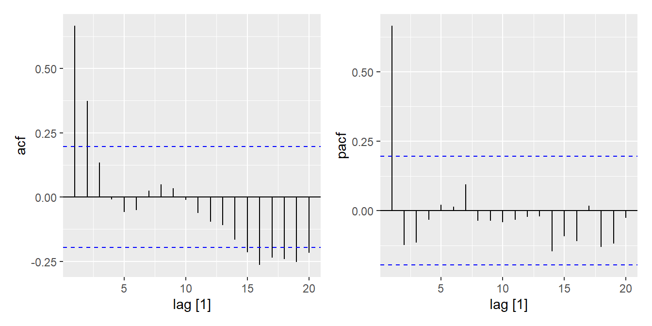
Recall that in our simulation, the residuals were modeled by an \(AR(1)\) process. So, it is not surprising that the residuals are correlated and that the partial autocorrelation function is only significant for the first lag.
Adding AR to the Model
The autocorrelation in the data shows that OLS is insufficient on its own. To fix it, we can add an AR(p) process to the residuals.
\[ y_t = \beta_0 + \beta_1 x_t + \eta_t \]
where \(\eta_t\) is an \(AR(p)\) error. Note that \(\eta_t\) can represent more than just \(AR\) processes, but we have specified it here as an \(AR(p)\).
Our above analysis identified an \(AR(1)\) process as appropriate. We also know this because the data was simulated. We can easily add that to the residuals with the following code.
lm_ar <- dat |>
  model(AR(x ~ Time + order(1))) # AR(1) fit to residuals of LM

tidy(lm_ar)| term | estimate | std.error | statistic | p.value |
|---|---|---|---|---|
| $\alpha_0$ | 22.1229022 | 5.4649024 | 4.048179 | 0.0001039 |
| Time | 0.9458886 | 0.2384769 | 3.966375 | 0.0001398 |
| ar1 | 0.6819469 | 0.0746126 | 9.139831 | 0.0000000 |
This model is a much better fit and gives more accurate errors and confidence levels.
Fitting a Regression Model to the Global Temperature Time Series
In Chapter 4 Lesson 4, we fit AR models to data representing the Earth’s mean annual temperature from 1880 to 2023. We assumed in that analysis that the entire series was a stochastic process, without a deterministic trend. In this section we will study how the same process could be modeled with a deterministic trend. The values of the series represent the deviation of the mean global surface temperature from the long-term average from 1951 to 1980. (Source: NASA/GISS.) We will consider the portion of the time series beginning in 1970.
Show the code
temps_ts <- rio::import("https://byuistats.github.io/timeseries/data/global_temparature.csv") |>
  as_tsibble(index = year) |>
  filter(year >= 1970)

temps_ts |> autoplot(.vars = change) +
    labs(
      x = "Year",
      y = "Temperature Change (Celsius)",
      title = paste0("Change in Mean Annual Global Temperature (", min(temps_ts$year), "-", max(temps_ts$year), ")")
    ) +
    theme_minimal() +
    theme(
      plot.title = element_text(hjust = 0.5)
    ) +
  geom_smooth(method='lm', formula= y~x)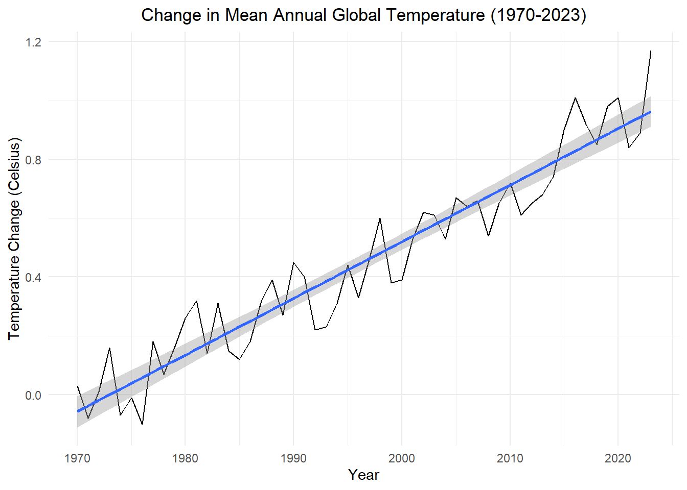
Visually, it is easy to spot a positive trend in these data. We model the data using
\[ x_t = \alpha_0 + \alpha_1 t + z_t \]
The following table shows the results of using OLS.
Show the code
global <- tibble(x = scan("https://byuistats.github.io/timeseries/data/global.dat")) |>
    mutate(
        date = seq(
            ymd("1856-01-01"),
            by = "1 months",
            length.out = n()),
        year = year(date),
        year_month = tsibble::yearmonth(date),
        stats_time = year + c(0:11)/12)

global_ts <- global |>
    as_tsibble(index = year_month)

temp_tidy <- global_ts |> filter(year >= 1970)
temp_lm <- temp_tidy |>
  model(lm = TSLM(x ~ stats_time ))
# tidy(temp_lm) |> pull(estimate)

tidy(temp_lm) |>
  select(-.model) |> # Remove the .model column
  mutate(
    # Relabel terms to use LaTeX
    term = case_when(
      term == "(Intercept)" ~ "$\\alpha_0$",
      term == "stats_time" ~ "$\\alpha_1$",
      TRUE ~ term
    ),
    lower = estimate + qnorm(0.025) * std.error,
    upper = estimate + qnorm(0.975) * std.error
  ) |>
display_table()| term | estimate | std.error | statistic | p.value | lower | upper |
|---|---|---|---|---|---|---|
| $\alpha_0$ | -34.920409 | 1.164899 | -29.97721 | 0 | -37.2035680 | -32.6372500 |
| $\alpha_1$ | 0.017654 | 0.000586 | 30.12786 | 0 | 0.0165055 | 0.0188025 |
The 95% confidence interval for the slope does not contain zero. If the errors were independent, this would be conclusive evidence that there is a significant linear relationship between the year and the global temperature. Remember that using OLS underestimates the standard error of the constant and slope term. In this case, the conclusion that temperatures are rising based on a statistically significant positive slope could be a mistake.
Table 4 presents an estimate of the ACF values for 10 monthly lags. Note that there is significant positive autocorrelation in the residual series for short lags. This implies that the standard errors will be underestimated, and the confidence interval is inappropriately narrow.
Here are the values of the autocorrelation and partial-autocorrelation functions of the residuals and the accompanying charts:
| type | 1M | 2M | 3M | 4M | 5M | 6M | 7M | 8M | 9M | 10M |
|---|---|---|---|---|---|---|---|---|---|---|
| ACF | 0.706 | 0.638 | 0.500 | 0.447 | 0.375 | 0.307 | 0.254 | 0.206 | 0.120 | 0.078 |
| PACF | 0.706 | 0.278 | -0.046 | 0.057 | 0.014 | -0.042 | -0.003 | -0.004 | -0.115 | -0.015 |
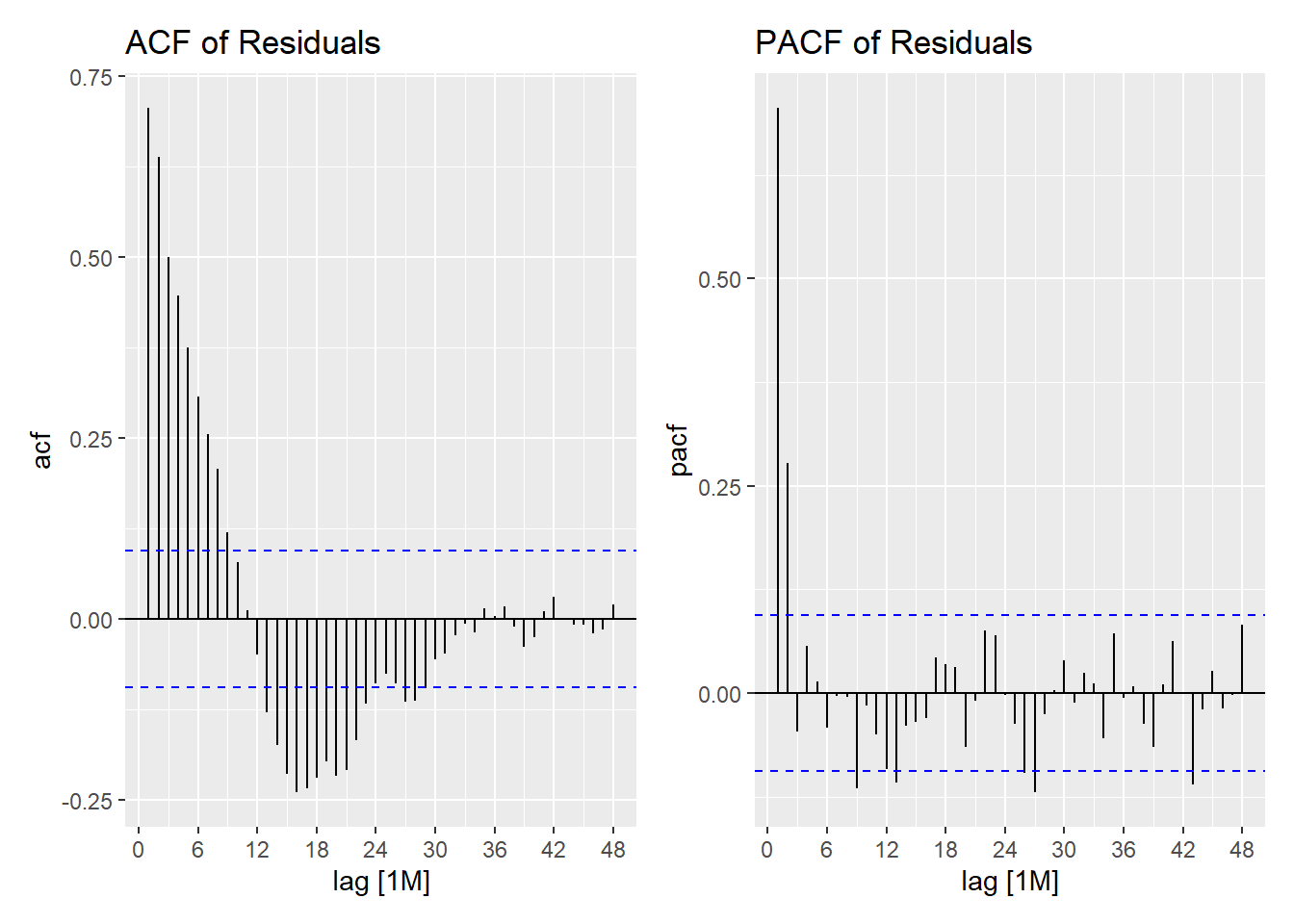
The PACF above shows 2 significant lags, so we will refit the linear model with an AR(2) process for the residuals.
lm_ar <- temp_tidy |>
  model(AR(x ~ stats_time + order(2))) # AR(2) fit to residuals of LM

tidy(lm_ar)| term | estimate | std.error | statistic | p.value |
|---|---|---|---|---|
| $\alpha_0$ | -7.6791790 | 1.4613752 | -5.254762 | 2e-07 |
| $\alpha_1$ | 0.0038818 | 0.0007377 | 5.262208 | 2e-07 |
| ar1 | 0.5000352 | 0.0462568 | 10.809982 | 0e+00 |
| ar2 | 0.2860945 | 0.0461051 | 6.205274 | 0e+00 |
This model is a much better fit and gives more accurate errors and confidence levels.
Class Activity: Linear Models with Seasonal Variables (10 min)
Some time series involve seasonal variables. In this section, we will address one way to include seasonality in a regression analysis of a time series. In the next lesson, we will explore another method.
Additive Seasonal Indicator Variables
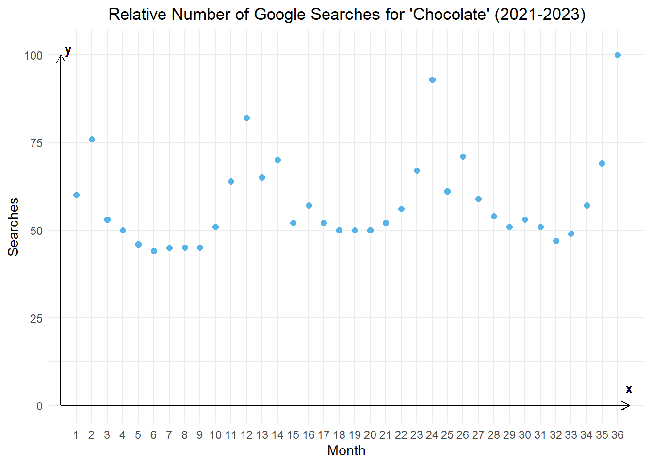
Recall the time series representing the monthly relative number of Google searches for the term “chocolate.” Here is a time plot of the data from 2021 to 2023. Month 1 is January 2021, month 13 is January 2022, and month 25 is January 2023.
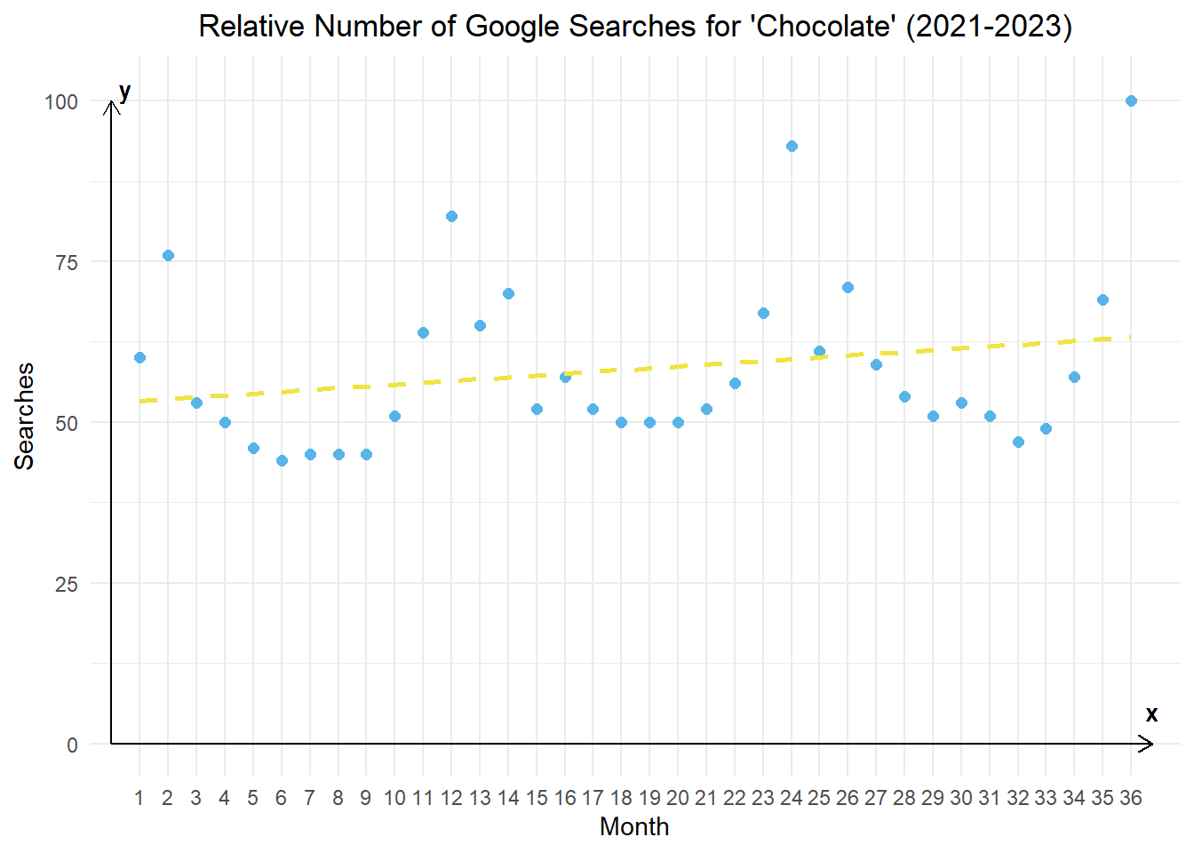
We fit a regression line to these data.
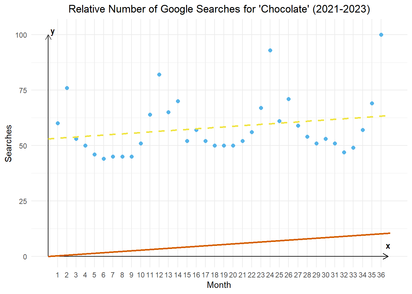
Now, we draw a line that is parallel to the regression line (has the same slope) but has a Y-intercept of 0.
For each month, we find the average amount that the relative number of google seachers that month deviates from the orange line (that is parallel to the regression line and passes through the origin). So, the length of the green line is the same for every January, etc.
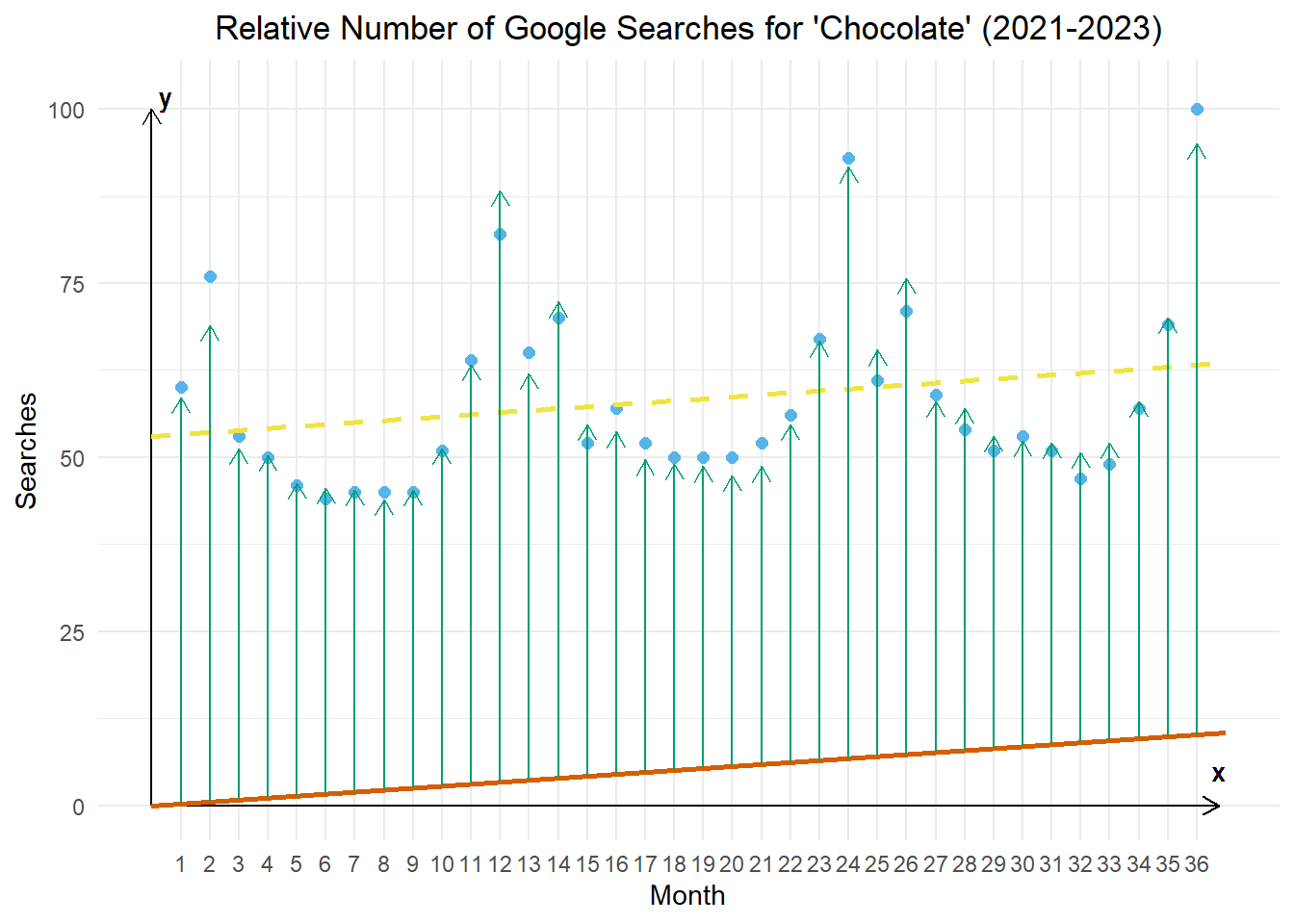
When the bottom of the green arrow is on the orange line, the top of the green arrow is the estimate of the value of the time series for that month.
We will create a linear model that includes a constant term for each month. This constant monthly term is called a seasonal indicator variable. This name is derived from the fact that each variable indicates (either as 1 or 0) whether a given month is represented. For example, one of the seasonal indicator variables will represent January. It will be equal to 1 for any value of \(t\) representing an observation drawn in January and 0 otherwise. Indicator variables are also called dummy varaibles.
This additive model with seasonal indicator variables can be perceived similarly to other additive models with a seasonal component:
\[ x_t = m_t + s_t + z_t \]
where \[ s_t = \begin{cases} \beta_1, & t ~\text{falls in season}~ 1 \\ \beta_2, & t ~\text{falls in season}~ 2 \\ ⋮~~~~ & ~~~~~~~~~~~~⋮ \\ \beta_s, & t ~\text{falls in season}~ s \end{cases} \]
and \(s\) is the number of seasons in one cycle/period, and \(n\) is the number of observations, so \(t = 1, 2, \ldots, n\) and \(i = 1, 2, \ldots, s\), and \(z_t\) is the residual error series, which can be autocorrelated.
It is important to note that \(m_t\) does not need to be a constant. It can be a linear trend: \[m_t = \alpha_0 + \alpha_1 t\] or quadratic: \[ m_t = \alpha_0 + \alpha_1 t + \alpha_2 t^2 \] a polynomial of degree \(p\): \[ m_t = \alpha_0 + \alpha_1 t + \alpha_2 t^2 + \cdots + \alpha_p t^p\]
or any other function of \(t\).
If \(s_t\) has the same value for all corresponding seasons, then we can write the model as: \[ x_t = m_t + \beta_{1 + [(t-1) \mod s]} + z_t \]
Putting this all together, if we have a time series that has no intercept (starts at the origin), a linear trend, and monthly observations where \(t=1\) corresponds to January, then the model becomes: \[ \begin{align*} x_t &= ~~~~ \alpha_1 t + s_t + z_t \\ &= \begin{cases} \alpha_1 t + \beta_1 + z_t, & t = 1, 13, 25, \ldots ~~~~ ~~(January) \\ \alpha_1 t + \beta_2 + z_t, & t = 2, 14, 26, \ldots ~~~~ ~~(February) \\ ~~~~~~~~⋮ & ~~~~~~~~~~~~⋮ \\ \alpha_1 t + \beta_{12} + z_t, & t = 12, 24, 36, \ldots ~~~~ (December) \end{cases} \end{align*} \] This is the model illustrated in Figure 8. The orange line represents the term \(\alpha_1 t\) and the green arrows represent the indicator seasonal variables with values of \(\beta_1, ~ \beta_2, ~ \ldots, ~ \beta_{12}\).
Note
In this model specification we set \(\alpha_0=0\), no intercept, so that the parameter estimates for \(\beta_1, ~ \beta_2, ~ \ldots, ~ \beta_{12}\) represent the levels of the seasonal values. We will explore a different specification below.
The folded chunk of code below fits the model to the data and computes the estimated parameter values.
Show the code
chocolate_month <- rio::import("https://byuistats.github.io/timeseries/data/chocolate.csv") |>
  mutate(
    dates = yearmonth(ym(Month)),
    month = month(dates),
    year = year(dates),
    # 'month_seq' is what we want: a time index starting from 1.
    month_seq = 1:n()
  ) |>
  # Set factor levels to get "Jan", "Feb", etc.
  mutate(month = factor(month, levels = 1:12, labels = month.abb)) |>
  as_tsibble(index = dates)


chocolate_lm <- chocolate_month |>
  model(TSLM(chocolate ~ 0 + month_seq + month))
The estimated value of the trend \(\alpha_1\) is 0.094. This suggests the search volume increases by about 0.094 units each month.
| Jan | Feb | Mar | Apr | May | Jun | Jul | Aug | Sep | Oct | Nov | Dec |
|---|---|---|---|---|---|---|---|---|---|---|---|
| 39.805 | 48.411 | 34.566 | 34.272 | 32.878 | 29.784 | 31.239 | 30.345 | 30.201 | 35.056 | 44.712 | 67.618 |
Now, we compute forecasted values for the relative number of Google searches for the word “Chocolate.”
Show the code
num_years_to_forecast <- 5
num_forecast_steps <- num_years_to_forecast * 12

last_date <- max(chocolate_month$dates)
last_month_seq <- max(chocolate_month$month_seq)

new_dat <- tibble(
  dates = seq(last_date, by = 1, length.out = num_forecast_steps + 1)[-1],
  month_seq = (last_month_seq + 1):(last_month_seq + num_forecast_steps),
  month = factor(month(dates, label = TRUE, abbr = TRUE), levels = month.abb)
) |>
  as_tsibble(index = dates)

# Generate the forecast by passing the new data
chocolate_forecast <- chocolate_lm |>
  forecast(new_data = new_dat)

# Plot the forecast
chocolate_forecast |>
  autoplot(chocolate_month, level = 95) +
  labs(
      x = "Month",
      y = "Relative Count of Google Searches",
      title = paste0("Google Searches for 'Chocolate' (", min(chocolate_month$year), "-", max(chocolate_month$year), ")"),
      subtitle = paste0(num_years_to_forecast, "-Year Forecast Based on a Linear Model with Seasonal Indicator Variables")
    ) +
    theme_minimal() +
    theme(
      plot.title = element_text(hjust = 0.5),
      plot.subtitle = element_text(hjust = 0.5)
    )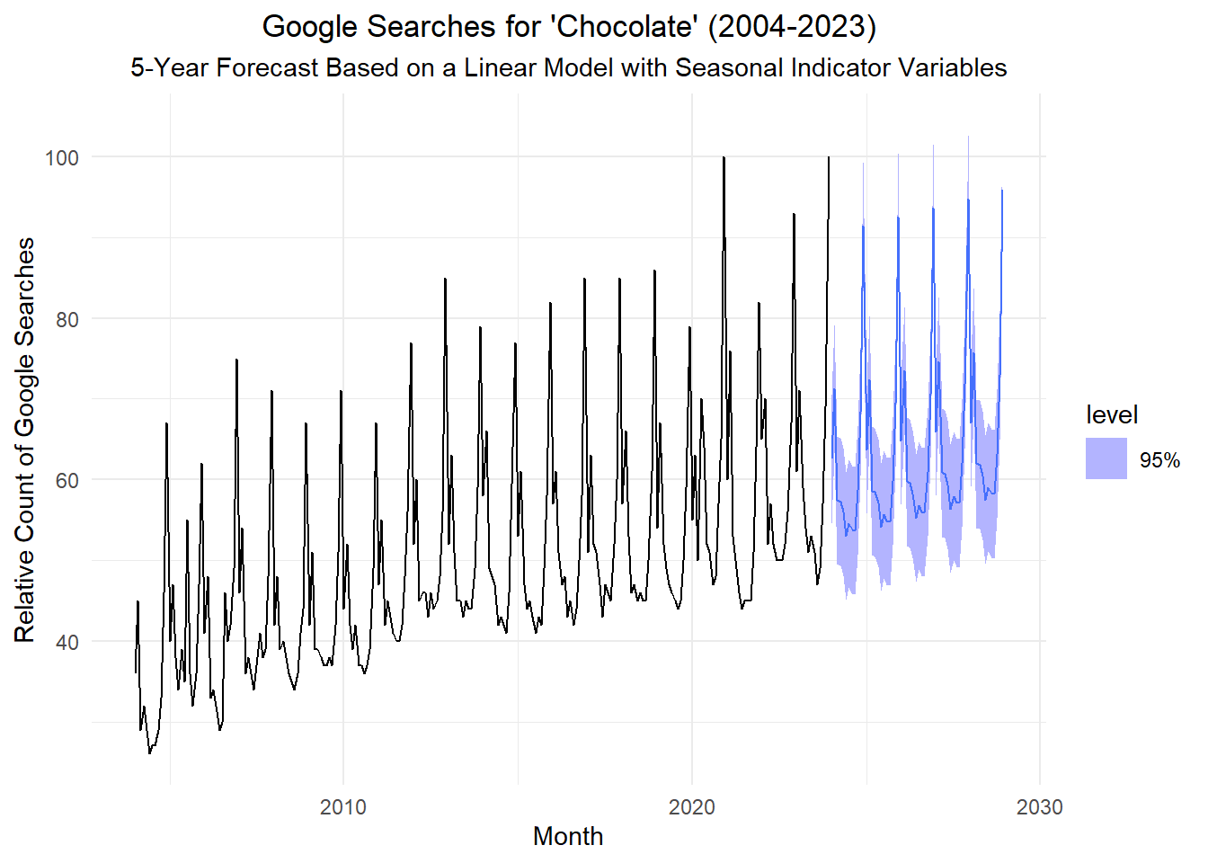
These are a subsample of the forecasted values.
Show the code
forecast_tbl <- chocolate_forecast |>
  as_tibble() |>
  select(dates, Forecast = .mean) |>
  mutate(
    dates = as.character(dates),
    Forecast = as.character(round(Forecast, 3))
  )

bind_rows(
  forecast_tbl |> head(4),
  tibble(dates = "...", Forecast = "..."),
  forecast_tbl |> tail(3)
) |>
knitr::kable(col.names = c("Date", "Forecast"))| Date | Forecast |
|---|---|
| 2024 Jan | 62.532 |
| 2024 Feb | 71.232 |
| 2024 Mar | 57.482 |
| 2024 Apr | 57.282 |
| … | … |
| 2028 Oct | 63.159 |
| 2028 Nov | 72.909 |
| 2028 Dec | 95.909 |
Additive Seasonal Indicator Variables with Reference Period
Recall the modeling choice of making the intercept zero in the previous section. That forces the estimates of \(\beta_i\) to be equal to the level of the seasonal values. There is an alternative specification that is often used that includes an intercept. When we include an overall intercept (\(\alpha_0\)), we must omit one of the seasonal indicator variables to avoid perfect multicollinearity (or the “dummy variable trap”). The omitted month (by default, R and TSLM will choose the first level, “January”) becomes the reference level. All other seasonal indicator variables (for February, March, etc.) will then represent the difference in the value of that period’s estimate compared to January (intercept).
Formally, the model with the intercept:
\[x_t = m_t + s_t + z_t\] where \(m_t\) represents the trend component and \(s_t\) represents the seasonal component.
For our model, the linear trend is:
\[m_t = \alpha_0 + \alpha_1 t\] And a seasonal component, \(s_t\), where all parameters are differences relative to January: \[ \begin{align*} x_t &= \alpha_0 + \alpha_1 t + s_t + z_t \\ &= \begin{cases} \alpha_0 +\alpha_1 t + \Delta\beta_2 + z_t, & t = 2, 14, 26, \ldots ~~~~ ~~(February) \\ \alpha_0 +\alpha_1 t + \Delta\beta_3 + z_t, & t = 3, 15, 27, \ldots ~~~~ ~~(March) \\ ~~~~~~~~⋮ & ~~~~~~~~~~~~⋮ \\ \alpha_0 +\alpha_1 t + \Delta\beta_{12} + z_t, & t = 12, 24, 36, \ldots ~~~~ (December) \end{cases} \end{align*} \]
In this model, the \(\alpha_0\) parameter is the intercept for January (the reference month) or \(\beta_1\) in the prior specification, and each \(\Delta\beta_i\) parameter is the difference between that month’s intercept and January’s. To obtain the estimate for the level for each period, we follow \(\beta_i=\alpha_0+\Delta\beta_i\)
Show the code
# Re-load the data (as done in the original file)
# This is to ensure the factor levels are set correctly for this chunk
chocolate_month <- rio::import("https://byuistats.github.io/timeseries/data/chocolate.csv") |>
mutate(
dates = yearmonth(ym(Month)),
month = month(dates),
year = year(dates),
month_seq = 1:n()
) |>
# Set factor levels to get "Jan", "Feb", etc.
# This makes "Jan" (month 1) the reference level by default
mutate(month = factor(month, levels = 1:12, labels = month.abb)) |>
as_tsibble(index = dates)

# Fit the model WITH an intercept
# TSLM(chocolate ~ month_seq + month)
# is equivalent to:
# TSLM(chocolate ~ 1 + month_seq + monthFeb + monthMar + ...)
chocolate_lm <- chocolate_month |>
model(TSLM(chocolate ~ month_seq + month))
The estimated value of the trend \(\alpha_1\) (term month_seq) is 0.094, equal to the previous model specification.
The estimated value of the overall intercept \(\alpha_0\) (term (Intercept)) is 39.805. This represents the intercept for January (the reference month), equal to \(\beta_1\) in the previous model specification.
The table below shows the estimates for the \(\Delta\beta_i\) parameters (differences relative to January) as well as the final calculated intercept for each month, \(\beta_i=\alpha_0 + \Delta\beta_i\). For example, the value for Feb (February) is 8.606. This means the estimate value for February is about 8.606 units higher than the value for January.
| Parameter | Jan | Feb | Mar | Apr | May | Jun | Jul | Aug | Sep | Oct | Nov | Dec |
|---|---|---|---|---|---|---|---|---|---|---|---|---|
| \(\alpha_0\), \(\Delta\beta_i\) | 39.805 | 8.606 | -5.239 | -5.533 | -6.927 | -10.022 | -8.566 | -9.460 | -9.604 | -4.749 | 4.907 | 27.813 |
| \(\beta_i\) | 39.805 | 48.411 | 34.566 | 34.272 | 32.878 | 29.784 | 31.239 | 30.345 | 30.201 | 35.056 | 44.712 | 67.618 |
Homework Preview (5 min)
- Review upcoming homework assignment
- Clarify questions