pacman::p_load(
  tidyverse,  # ggplot, mutate(), cleaning...
  tsibble,    # as_tsibble()
  fable,      # model(...), forecast(), tidy(), glance()...
  feasts,     # ACF(), PACF()
  ggtime,     # autoplot() for tsibbles
  patchwork,  # + and / for ggplots
  rio         # import()
)Autocorrelation Concepts
Chapter 2: Lesson 2
Learning Outcomes
Define key terms in time series analysis
- Define the ensemble of a time series
- Define the expected value (or mean function) of a time series model
- Define the sample estimate of the population mean of a time series
- Define the variance function of a time series model
- State the constant variance estimator for a time series model
- Explain the stationarity assumption
- Explain the stationary variance assumption
- Define lag
- Define autocorrelation
- Define the second-order stationary time series
- Explain the autocovariance function in Equation (2.11)
- Explain the lag k autocorrelation function in Equation (2.12)
- Define the autocovariance function, acvf
- Define the sample autocorrelation function, acf
Calculate sample estimates of autocovariance and autocorrelation functions from time series data
- Define the sample autocovariance function, c_k
- Define the sample autocorrelation function, r_k
Preparation
- Read Sections 2.2.5
Learning Journal Exchange (10 min)
- Review another student’s journal
- What would you add to your learning journal after reading your partner’s?
- What would you recommend your partner add to their learning journal?
- Sign the Learning Journal review sheet for your peer
Packages
Note: the MASS package causes conflicts with tidyverse. Click below if you have code issues.
Hands-on Exercise – Exploring Sample Autocorrelation (40 min)
Comparison of Independent and Autocorrelated Error Terms
In the previous lesson, we computed the sample covariance and sample correlation coefficient between two independent variables. When working with time series, the observations are not independent. There is often a relationship between sequential observations. We will compute the autocovariance function and autocorrelation function for a time series. Note: the prefix “auto” comes from a Greek root meaning “self.”
The figure below illustrates the difference between a series of data, where the residuals are independent compared to a series with autocorrelated data.
Autocovariance and Autocorrelation
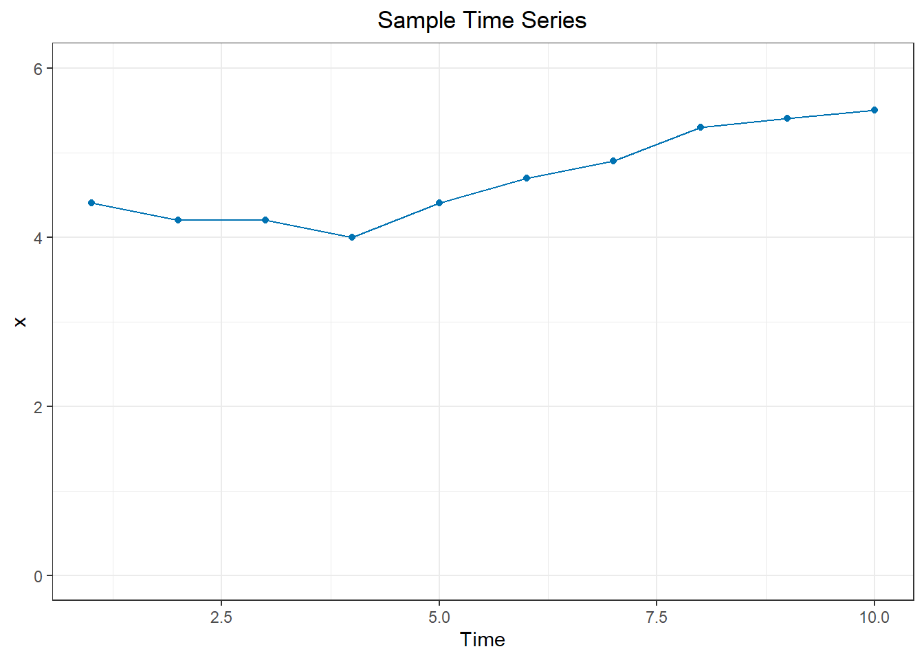
We will use the following data to explore the concepts of autovariance and autocorrelation.
| t | $$ x_t $$ |
|---|---|
| 1 | 4.4 |
| 2 | 4.2 |
| 3 | 4.2 |
| 4 | 4.0 |
| 5 | 4.4 |
| 6 | 4.7 |
| 7 | 4.9 |
| 8 | 5.3 |
| 9 | 5.4 |
| 10 | 5.5 |
You can use this R command to read in the observations.
x <- c( 4.4, 4.2, 4.2, 4, 4.4, 4.7, 4.9, 5.3, 5.4, 5.5 )
We will use the sample mean of these data repeatedly. The value of \(\bar x\) is:
\[ \bar x = \frac{1}{n} \sum\limits_{t=1}^{n} x_t = \frac{1}{10} \cdot 47 = 4.7 \]
We will be finding the autocovariance and correlation of a time series with itself. First, we start with a lag of 1. With a lag of 1 the corresponding values of the time series that are being compared are shifted by one time unit. Then, we will consider any integer lag: lag \(k\).
Lag \(k\) Sample Autocovariance Function (acvf), \(c_k\)
The lag \(k\) sample autocovariance function, acvf, denoted \(c_k\), is defined as
\[ c_k = \frac{1}{n} \sum\limits_{t=1}^{n-k}(x_t-\bar x)(x_{t+k}-\bar x) \]
We denote the lag by the letter \(k\), where \(k \ge 0\). This is the number of values the data set is shifted to compute the autocovariance.
Lag \(k=1\) Sample Autocovariance Function, \(c_1\)
We will now find the autocovariance between the values in a time series (\(x = x_t\)) and the same values, shifted by one unit of time (\(y = x_{t+1}\)).
| t | $$ x_t $$ | $$ x_{t+1} $$ | $$ x_t-\bar x $$ | $$ (x_t-\bar x)^2 $$ | $$ x_{t+1}-\bar x$$ | $$ (x-\bar x)(x_{t+1}-\bar x) $$ |
|---|---|---|---|---|---|---|
| 1 | 4.4 | 4.2 | -0.3 | 0.09 | -0.5 | 0.15 |
| 2 | 4.2 | 4.2 | -0.5 | 0.25 | -0.5 | 0.25 |
| 3 | 4.2 | 4 | -0.5 | 0.25 | -0.7 | 0.35 |
| 4 | 4 | 4.4 | -0.7 | 0.49 | -0.3 | 0.21 |
| 5 | 4.4 | 4.7 | -0.3 | 0.09 | 0 | 0 |
| 6 | 4.7 | 4.9 | 0 | 0 | 0.2 | 0 |
| 7 | 4.9 | 5.3 | 0.2 | 0.04 | 0.6 | 0.12 |
| 8 | 5.3 | 5.4 | 0.6 | 0.36 | 0.7 | 0.42 |
| 9 | 5.4 | 5.5 | 0.7 | 0.49 | 0.8 | 0.56 |
| 10 | 5.5 | — | 0.8 | 0.64 | — | — |
| sum | 47 | 42.6 | 0 | 2.7 | 0.3 | 2.06 |
The scatterplot below illustrates the relationship between the observed data (\(x_t\)) and the next observation (\(x_{t+1}\)).
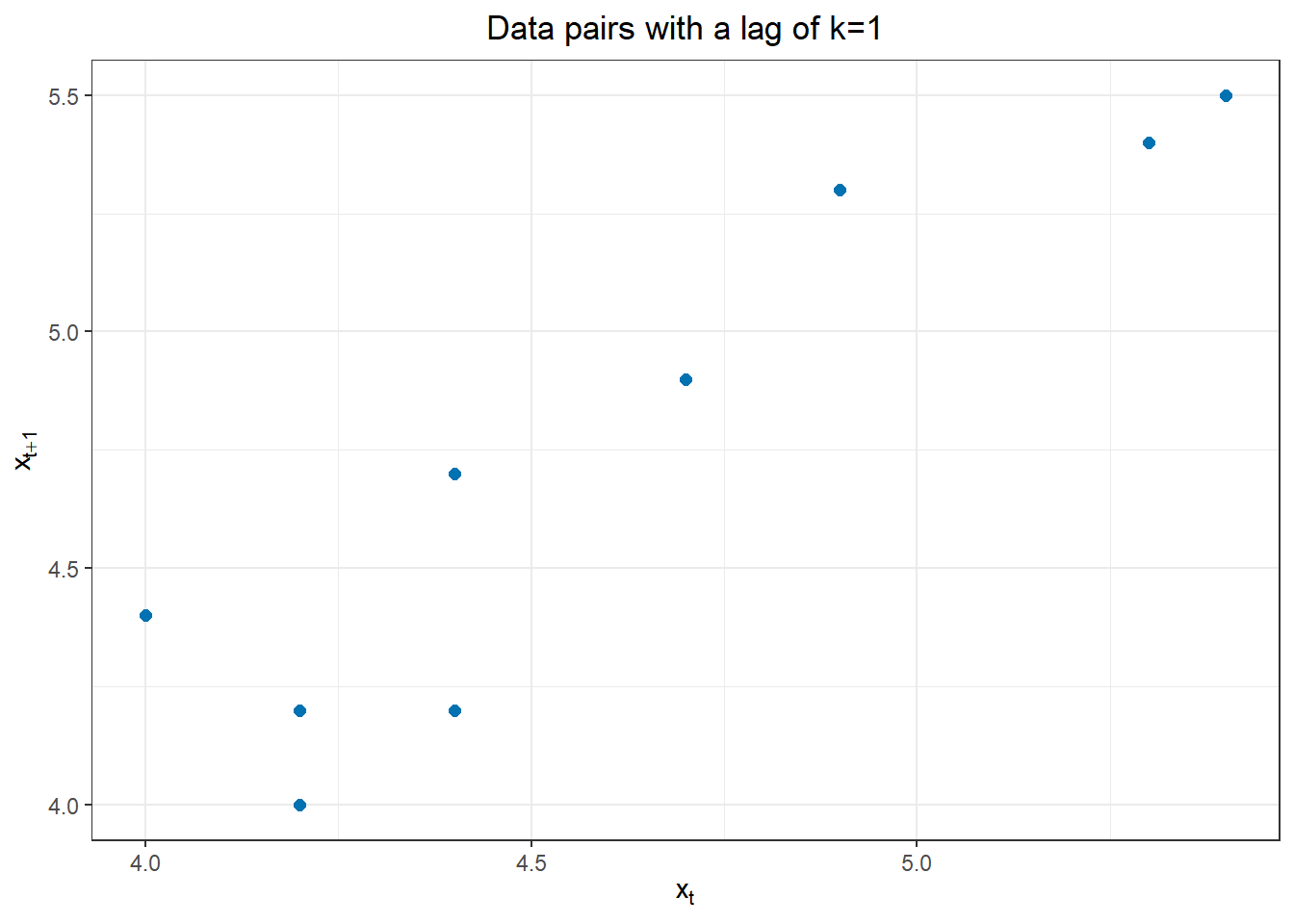
In this example, the second variable is \(x_{t+1}\), where \(t>1\). the autocovariance of \(x_t\) and \(x_{t+1}\) is:
\[ c_1 = \frac{1}{n} \sum\limits_{t=1}^{n-1}(x_t-\bar x)(x_{t+1}-\bar x) = \frac{1}{10} \sum\limits_{t=1}^{9}(x_t-\bar x)(x_{t+1}-\bar x) = \frac{1}{10} \cdot 2.06 = 0.206 \]
This is the (auto)covariance of \(x\) with itself, but with a lag of 1 time unit. This is the value of the lag \(k=1\) autocovariance function, acvf_1.
Lag \(k\) Sample Autocorrelation Function (acf), \(r_k\)
The sample autocorrelation function, acf, denoted \(r_k\), where \(k\) is the lag, is defined as
\[ r_k = \frac{c_k}{c_0} = \frac{ \frac{1}{n} \sum\limits_{t=1}^{n-k}(x_t-\bar x)(x_{t+k}-\bar x) }{ \frac{1}{n} \sum\limits_{t=1}^{n}(x_t-\bar x)^2 } = \frac{ \sum\limits_{t=1}^{n-k}(x_t-\bar x)(x_{t+k}-\bar x) }{ \sum\limits_{t=1}^{n}(x_t-\bar x)^2 } \]
Note that \(c_0\) is the variance of \(x\), but computed by dividing by \(n\), instead of \(n-1\).
Lag \(k=1\) Sample Autocorrelation Function, \(r_1\)
We can compute the lag 1 autocorrelation or the autocorrelation of \(x\) with lag 1 as the quotient \(r_1 = \frac{c_1}{c_0}\). We have already determined that \(c_1 = 0.206\). We now compute \(c_0\):
\[ c_0 = \frac{1}{n} \sum\limits_{t=1}^{n-0} (x_t-\bar x)(x_{t+0}-\bar x) = \frac{1}{n} \sum\limits_{t=1}^{n} (x_t-\bar x)^2 = \frac{1}{10} \cdot 2.7 = 0.27 \]
We use \(c_0\) and \(c_1\) to compute \(r_1\). Here are two ways we can compute this value:
\[\begin{align*} r_1 &= \frac{c_1}{c_0} = \frac{ \frac{1}{n} \sum\limits_{t=1}^{9}(x_t-\bar x)(x_{t+1}-\bar x) }{ \frac{1}{n} \sum\limits_{t=1}^{10}(x_t-\bar x)^2 } = \frac{ \frac{1}{10} \cdot 2.06 }{ \frac{1}{10} \cdot 2.7 } = \frac{0.206}{0.27} = 0.763 \\ &= \frac{ \sum\limits_{t=1}^{9}(x_t-\bar x)(x_{t+1}-\bar x) }{ \sum\limits_{t=1}^{10}(x_t-\bar x)^2 } = \frac{2.06}{2.7} = 0.763 \end{align*}\]
- What does the lag 1 autocorrelation, \(c_1\), measure?
Lag \(k = 2\)
| t | $$ x_t $$ | $$ x_{t+k} $$ | $$ x_t-\bar x $$ | $$ (x_t-\bar x)^2 $$ | $$ x_{t+k}-\bar x$$ | $$ (x-\bar x)(x_{t+k}-\bar x) $$ |
|---|---|---|---|---|---|---|
| 1 | 4.4 | 4.2 | -0.3 | 0.09 | -0.5 | 0.15 |
| 2 | 4.2 | 4 | -0.5 | 0.25 | -0.7 | 0.35 |
| 3 | 4.2 | 4.4 | -0.5 | 0.25 | -0.3 | 0.15 |
| 4 | 4 | |||||
| 5 | 4.4 | |||||
| 6 | 4.7 | |||||
| 7 | 4.9 | 5.4 | 0.2 | 0.04 | 0.7 | 0.14 |
| 8 | 5.3 | 5.5 | 0.6 | 0.36 | 0.8 | 0.48 |
| 9 | 5.4 | — | 0.7 | 0.49 | — | — |
| 10 | 5.5 | — | 0.8 | 0.64 | — | — |
| sum | 47 |
The figure below illustrates the relationship between \(x_t\) and \(x_{t+2}\).
Lag \(k = 3\)
| t | $$ x_t $$ | $$ x_{t+k} $$ | $$ x_t-\bar x $$ | $$ (x_t-\bar x)^2 $$ | $$ x_{t+k}-\bar x$$ | $$ (x-\bar x)(x_{t+k}-\bar x) $$ |
|---|---|---|---|---|---|---|
| 1 | 4.4 | 4 | -0.3 | 0.09 | -0.7 | 0.21 |
| 2 | 4.2 | 4.4 | -0.5 | 0.25 | -0.3 | 0.15 |
| 3 | 4.2 | 4.7 | -0.5 | 0.25 | 0 | 0 |
| 4 | 4 | 4.9 | -0.7 | 0.49 | 0.2 | -0.14 |
| 5 | 4.4 | 5.3 | -0.3 | 0.09 | 0.6 | -0.18 |
| 6 | 4.7 | 5.4 | 0 | 0 | 0.7 | 0 |
| 7 | 4.9 | 5.5 | 0.2 | 0.04 | 0.8 | 0.16 |
| 8 | 5.3 | — | 0.6 | 0.36 | — | — |
| 9 | 5.4 | — | 0.7 | 0.49 | — | — |
| 10 | 5.5 | — | 0.8 | 0.64 | — | — |
| sum | 47 | 34.2 | 0 | 2.7 | 1.3 | 0.2 |
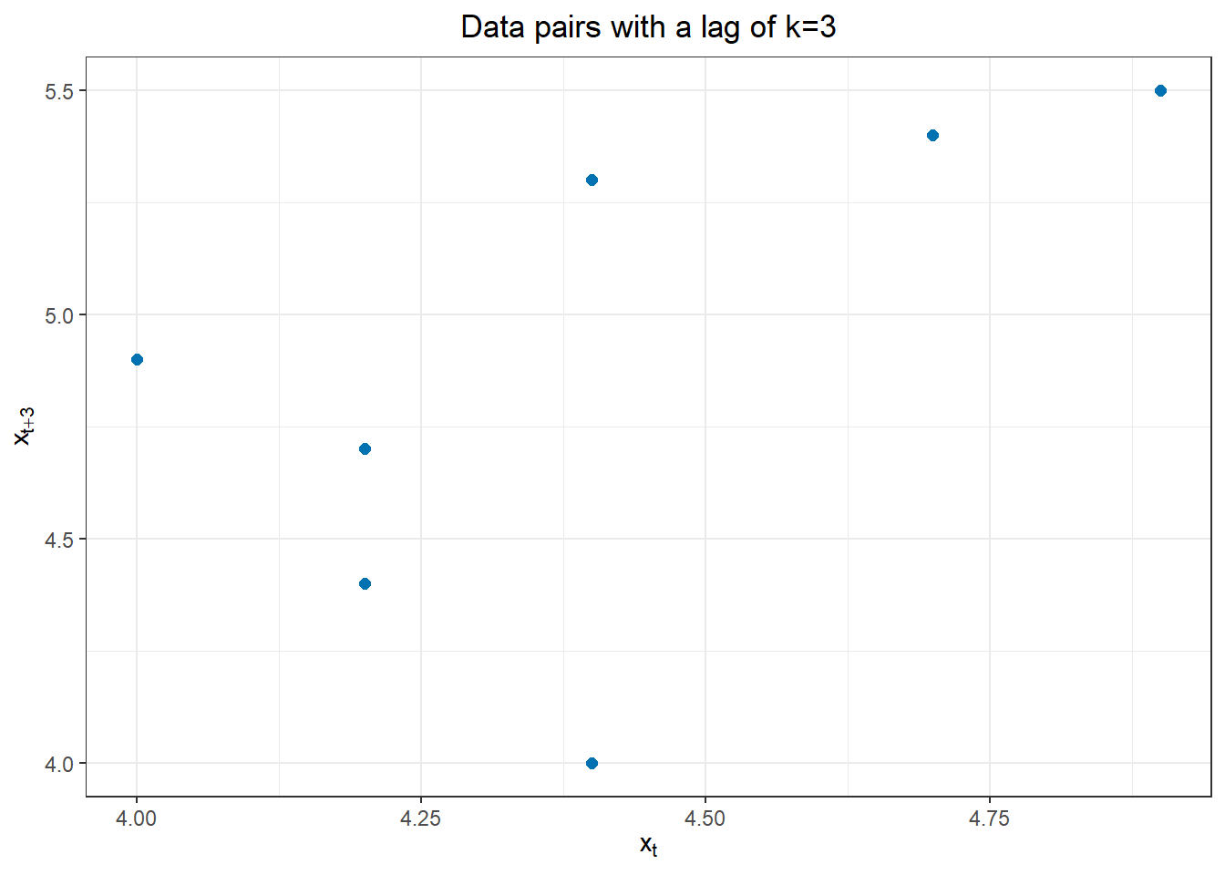
The figure below illustrates the correlations between \(x_t\) and \(x_{t+3}\). Note that \(c_3 = \dfrac{0.2}{10} = 0.02\) and \(r_3 = \dfrac{0.02}{0.27} = 0.0741\).
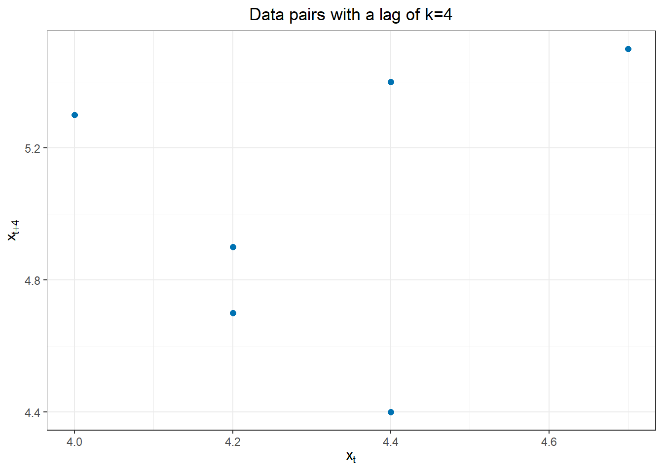
Lag \(k = 4\)
| t | $$ x_t $$ | $$ x_{t+k} $$ | $$ x_t-\bar x $$ | $$ (x_t-\bar x)^2 $$ | $$ x_{t+k}-\bar x$$ | $$ (x-\bar x)(x_{t+k}-\bar x) $$ |
|---|---|---|---|---|---|---|
| 1 | 4.4 | |||||
| 2 | 4.2 | |||||
| 3 | 4.2 | |||||
| 4 | 4 | |||||
| 5 | 4.4 | |||||
| 6 | 4.7 | |||||
| 7 | 4.9 | |||||
| 8 | 5.3 | |||||
| 9 | 5.4 | |||||
| 10 | 5.5 | |||||
| sum | 47 |
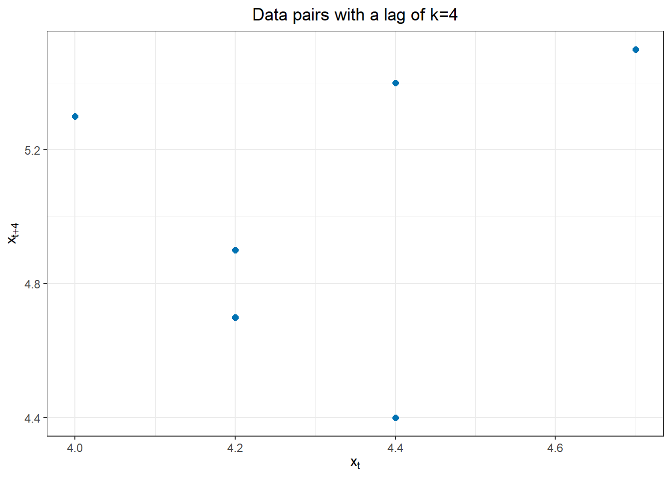
The figure below illustrates the correlations between \(x_t\) and \(x_{t+4}\).
Class Activity: Using R to compute the acvf and acf (5 min)
We will continue to use the following sample data.
 x <- c( 4.4, 4.2, 4.2, 4, 4.4, 4.7, 4.9, 5.3, 5.4, 5.5 )
 df <- data.frame(x = x)
acvf
This code gives the values of the acvf.
acf(df$x, plot=FALSE, type = "covariance")
Autocovariances of series 'df$x', by lag

     0      1      2      3      4      5      6      7      8      9
 0.270  0.206  0.121  0.020 -0.064 -0.113 -0.127 -0.093 -0.061 -0.024
acf
We can obtain the acf by changing the argument for the paramter type to "correlation".
acf(df$x, plot=FALSE, type = "correlation")
Autocorrelations of series 'df$x', by lag

     0      1      2      3      4      5      6      7      8      9
 1.000  0.763  0.448  0.074 -0.237 -0.419 -0.470 -0.344 -0.226 -0.089
Homework Preview (5 min)
- Review upcoming homework assignment
- Clarify questions