pacman::p_load(
  tidyverse,  # ggplot, mutate(), cleaning...
  tsibble,    # as_tsibble()
  fable,      # model(...), forecast(), tidy(), glance()...
  feasts,     # ACF(), PACF()
  ggtime,     # autoplot() for tsibbles
  patchwork,  # + and / for ggplots
  rio         # import()
)Holt-Winters Method (Multiplicative Models)
Chapter 3: Lesson 5
Learning Outcomes
Implement the Holt-Winter method to forecast time series
- Explain the Holt-Winters method equations for multiplicative decomposition models
- Explain the purpose of the paramters \(\alpha\), \(\beta\), and \(\gamma\)
- Interpret the coefficient estimates \(a_t\), \(b_t\), and \(s_t\) of the Holt-Winters smoothing algorithm
- Explain the Holt-Winters forecasting equation for multiplicative decomposition models, Equation (3.23)
- Use HoltWinters() to forecast multiplicative model time series
- Plot the Holt-Winters decomposition of a TS (see Fig 3.10)
- Plot the Holt-Winters fitted values versus the original time series (see Fig 3.11)
- Superimpose plots of the Holt-Winters predictions with the time series realizations (see Fig 3.13)
Preparation
- Read Sections 3.4.2-3.4.3, 3.5
Learning Journal Exchange (10 min)
Review another student’s journal
What would you add to your learning journal after reading another student’s?
What would you recommend the other student add to their learning journal?
Sign the Learning Journal review sheet for your peer
Packages
Class Discussion: Multiplicative Seasonality (10 min)
We can assume either additive or multiplicative seasonality. In the previous two lessons, we explored additive seasonality. In this lesson, we consider the case where the seasonality is multiplicative.
Additive seasonality is appropriate when the variation in the time series is roughly constant for any level. We assume multiplicative seasonality when the variation gets larger as the level increases.
Forecasting
Here are the forecasting equations we use, based on the model that is appropriate for the time series.
| Additive Seasonality | Multiplicative Seasonality | |
|---|---|---|
| Additive Slope | \[ \hat x_{n+k \mid n} = \left( a_n + k \cdot b_n \right) + s_{n+k-p} \] | \[ \hat x_{n+k \mid n} = \left( a_n + k \cdot b_n \right) \cdot s_{n+k-p} \] |
Update Equations (Multiplicative Seasonals)
The update equations for the seasonals are:
\[\begin{align*} a_t &= \alpha \left( \frac{x_t}{s_{t-p}} \right) + (1-\alpha) \left( a_{t-1} + b_{t-1} \right) && \text{Level} \\ b_t &= \beta \left( a_t - a_{t-1} \right) + (1-\beta) b_{t-1} && \text{Slope} \\ s_t &= \gamma \left( \frac{x_t}{a_{t}} \right) + (1-\gamma) s_{t-p} && \text{Seasonal} \end{align*}\]
Note that when the seasonal effect is additive, we subtract it from the time series to remove its effect. If the seasonal effect is multiplicative, we divide.
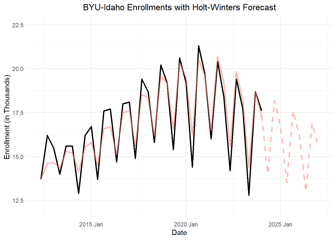
Small Group Activity: Holt-Winters Model for BYU-Idaho Enrollment Data (25 min)
We will now apply Holt-Winters filtering to the BYU-Idaho Enrollment data. First, we examine the time plot in Figure 1.
Show the code
# read in the data from a csv and make the tsibble
byui_enrollment_ts <- rio::import("https://byuistats.github.io/timeseries/data/byui_enrollment_2012.csv") |>
  rename(
    semester = "TermCode",
    year = "Year",
    enrollment = "On Campus Enrollment (Campus HC)"
  ) |>
  mutate(
    term =
      case_when(
        left(semester, 2) == "WI" ~ 1,
        left(semester, 2) == "SP" ~ 2,
        left(semester, 2) == "FA" ~ 3,
        TRUE ~ NA
      )
  ) |>
  filter(!is.na(term)) |>
  mutate(dates = yearmonth( ym( paste(year, term * 4 - 3) ) ) ) |>
  mutate(enrollment_1000 = enrollment / 1000) |>
  dplyr::select(semester, dates, enrollment_1000) |>
  as_tsibble(index = dates)

byui_enrollment_ts_expanded <- byui_enrollment_ts |>
  as_tibble() |>
  hw_additive_slope_multiplicative_seasonal_rounded("dates", "enrollment_1000", p = 3, predict_periods = 9) |>
  mutate(xhat_t = ifelse(t %in% c(1:36), round(a_t * s_t, 1), xhat_t)) |>
  select(-dates, -enrollment_1000)

# This is hard-coded for this data set, because I am in a hurry to get done.
# This revises the semester codes
byui_enrollment_ts_expanded$semester[1:3] <- c("SP11", "FA11", "WI12")
byui_enrollment_ts_expanded$semester[40:48] <- c("SP24", "FA24", "WI25",
                                                 "SP25", "FA25", "WI26",
                                                 "SP26", "FA26", "WI27")

byui_enrollment_ts_expanded |>
  tail(nrow(byui_enrollment_ts_expanded) - 3) |>
  ggplot(aes(x = date, y = x_t)) +
    geom_line(color = "black", linewidth = 1) +
    coord_cartesian(ylim = c(0, 22.5)) +
    labs(
      x = "Date",
      y = "Enrollment (in Thousands)",
      title = "BYU-Idaho On-Campus Enrollments (in Thousands)",
      color = "Components"
    ) +
    theme_minimal() +
    theme(legend.position = "none") +
    theme(plot.title = element_text(hjust = 0.5))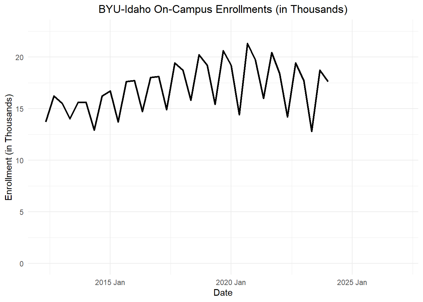
Table 1 summarizes the intermediate values for Holt-Winters filtering with multiplicative seasonals.
| $$Semester$$ | $$t$$ | $$x_t$$ | $$a_t$$ | $$b_t$$ | $$s_t$$ | $$\hat x_t$$ |
|---|---|---|---|---|---|---|
| SP11 | -2 | — | — | — | — | |
| FA11 | -1 | — | — | — | — | |
| WI12 | 0 | — | — | — | — | |
| SP12 | 1 | 13.7 | ||||
| FA12 | 2 | 16.2 | 14.2 | 0.082 | 1.03 | 14.6 |
| WI13 | 3 | 15.5 | 14.5 | 0.126 | 1.01 | 14.6 |
| SP13 | 4 | 14 | 14.5 | 0.101 | 0.99 | 14.4 |
| FA13 | 5 | 15.6 | 14.7 | 0.121 | 1.04 | 15.3 |
| WI14 | 6 | 15.6 | ||||
| SP14 | 7 | 12.9 | ||||
| FA14 | 8 | 16.2 | 14.8 | 0.08 | 1.05 | 15.5 |
| WI15 | 9 | 16.7 | 15.2 | 0.144 | 1.04 | 15.8 |
| SP15 | 10 | 13.7 | 15.1 | 0.095 | 0.96 | 14.5 |
| FA15 | 11 | 17.6 | 15.5 | 0.156 | 1.07 | 16.6 |
| ⋮ | ⋮ | ⋮ | ⋮ | ⋮ | ⋮ | ⋮ |
| FA21 | 29 | 20.4 | 18.5 | 0.086 | 1.12 | 20.7 |
| WI22 | 30 | 18.4 | 18.3 | 0.029 | 1.05 | 19.2 |
| SP22 | 31 | 14.2 | 17.9 | -0.057 | 0.87 | 15.6 |
| FA22 | 32 | 19.4 | 17.7 | -0.086 | 1.12 | 19.8 |
| WI23 | 33 | 17.7 | 17.5 | -0.109 | 1.04 | 18.2 |
| SP23 | 34 | 12.8 | 16.9 | -0.207 | 0.85 | 14.4 |
| FA23 | 35 | 18.7 | 16.7 | -0.206 | 1.12 | 18.7 |
| WI24 | 36 | 17.6 | 16.6 | -0.185 | 1.04 | 17.3 |
| SP24 | 37 | — | — | — | ||
| FA24 | 38 | — | — | — | ||
| WI25 | 39 | — | — | — | ||
| SP25 | 40 | — | — | — | ||
| FA25 | 41 | — | — | — | 1.12 | 17.6 |
| WI26 | 42 | — | — | — | 1.04 | 16.1 |
Small Group Activity: Applying Holt-Winters in R to the Apple Quarterly Revenue Data (10 min)
Recall the Apple, Inc., revenue values reported by Bloomberg:
Show the code
apple_ts <- rio::import("https://byuistats.github.io/timeseries/data/apple_revenue.csv") |>
  mutate(
    dates = mdy(date),
    year = lubridate::year(dates),
    quarter = lubridate::quarter(dates),
    value = revenue_billions
  ) |>
  dplyr::select(dates, year, quarter, value)  |>
  arrange(dates) |>
  mutate(index = tsibble::yearquarter(dates)) |>
  as_tsibble(index = index) |>
  dplyr::select(index, dates, year, quarter, value) |>
  rename(revenue = value) # rename value to emphasize data context

apple_ts |>
  autoplot(.vars = revenue) +
  labs(
    x = "Quarter",
    y = "Apple Revenue, Billions $US",
    title = "Apple's Quarterly Revenue, Billions of U.S. Dollars"
  ) +
  theme_minimal() +
  theme(plot.title = element_text(hjust = 0.5))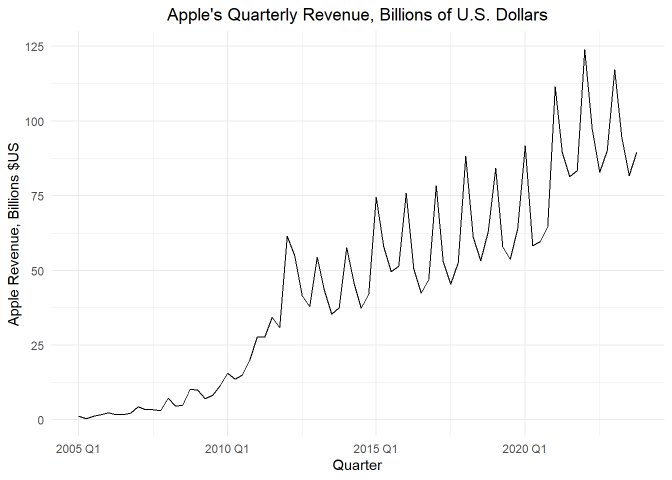
Here are a few rows of the summarized data.
| index | dates | year | quarter | revenue |
|---|---|---|---|---|
| 2005 Q1 | 2005-01-25 | 2005 | 1 | 1.24 |
| 2005 Q2 | 2005-04-25 | 2005 | 2 | 0.48 |
| 2005 Q3 | 2005-07-25 | 2005 | 3 | 1.24 |
| 2005 Q4 | 2005-10-30 | 2005 | 4 | 1.71 |
| 2006 Q1 | 2006-01-25 | 2006 | 1 | 2.42 |
| 2006 Q2 | 2006-04-25 | 2006 | 2 | 1.71 |
| ⋮ | ⋮ | ⋮ | ⋮ | ⋮ |
| 2023 Q2 | 2023-05-04 | 2023 | 2 | 94.836 |
| 2023 Q3 | 2023-08-03 | 2023 | 3 | 81.797 |
| 2023 Q4 | 2023-11-02 | 2023 | 4 | 89.498 |
We apply Holt-Winters filtering to the quarterly Apple revenue data with a multiplicative model:
Show the code
apple_hw <- apple_ts |>
  # tsibble::fill_gaps() |>
  model(Additive = ETS(revenue ~
        trend("A") +
        error("A") +
        season("M"),
        opt_crit = "amse", nmse = 1))
report(apple_hw)
Series: revenue
Model: ETS(A,A,M)
Smoothing parameters:
alpha = 0.8465418
beta = 0.0142208
gamma = 0.0001000036
Initial states:
l[0] b[0] s[0] s[-1] s[-2] s[-3]
0.05455891 -0.0543255 1.003384 0.9450199 1.100051 0.9515453
sigma^2: 32.8701
AIC AICc BIC
604.1173 606.8446 625.0939 We can compute some values to assess the fit of the model:
Show the code
# SS of random terms
sum(components(apple_hw)$remainder^2, na.rm = T)

# RMSE
forecast::accuracy(apple_hw)$RMSE

# Standard devation of the quarterly revenues
sd(apple_ts$revenue)- The sum of the square of the random terms is: 2235.1651229.
- The root mean square error (RMSE) is: 5.423105.
- The standard deviation of the number of incidents each month is 33.0205.
Figure 2 illustrates the Holt-Winters decomposition of the Apple revenue data.
Show the code
autoplot(components(apple_hw))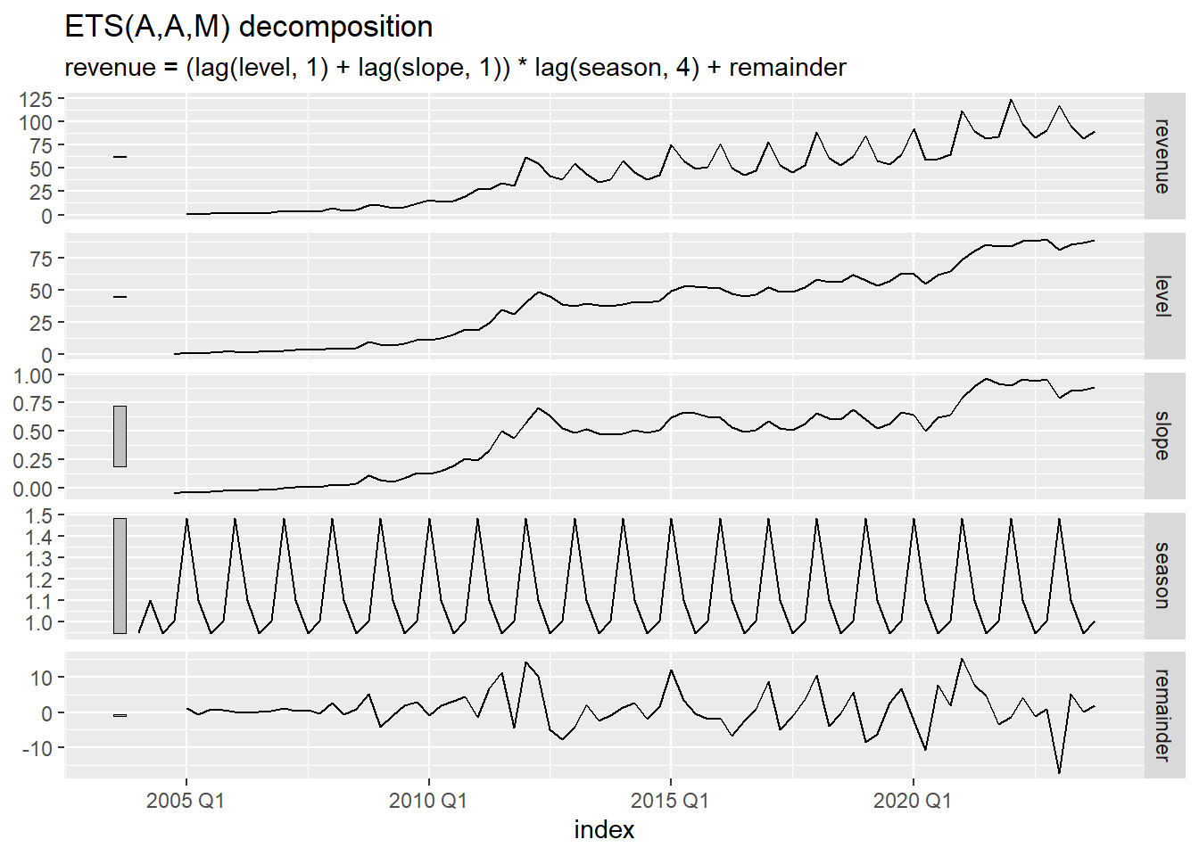
In Figure 3, we can observe the relationship between the Holt-Winters filter and the Apple revenue time series.
Show the code
augment(apple_hw) |>
  ggplot(aes(x = index, y = revenue)) +
    geom_line() +
    geom_line(aes(y = .fitted, color = "Fitted")) +
    labs(color = "")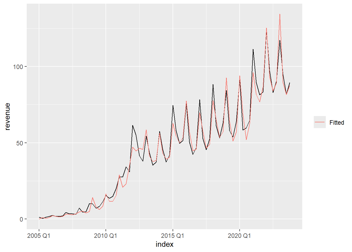
Figure 4 contains the information from Figure 3, with the addition of an additional four years of forecasted values. The light blue bands give a 95% prediction bands for the forecast.
Show the code
apple_forecast <- apple_hw |>
  forecast(h = "4 years")

apple_forecast |>
  autoplot(apple_ts, level = 95) +
  geom_line(aes(y = .fitted, color = "Fitted"),
    data = augment(apple_hw)) +
  scale_color_discrete(name = "")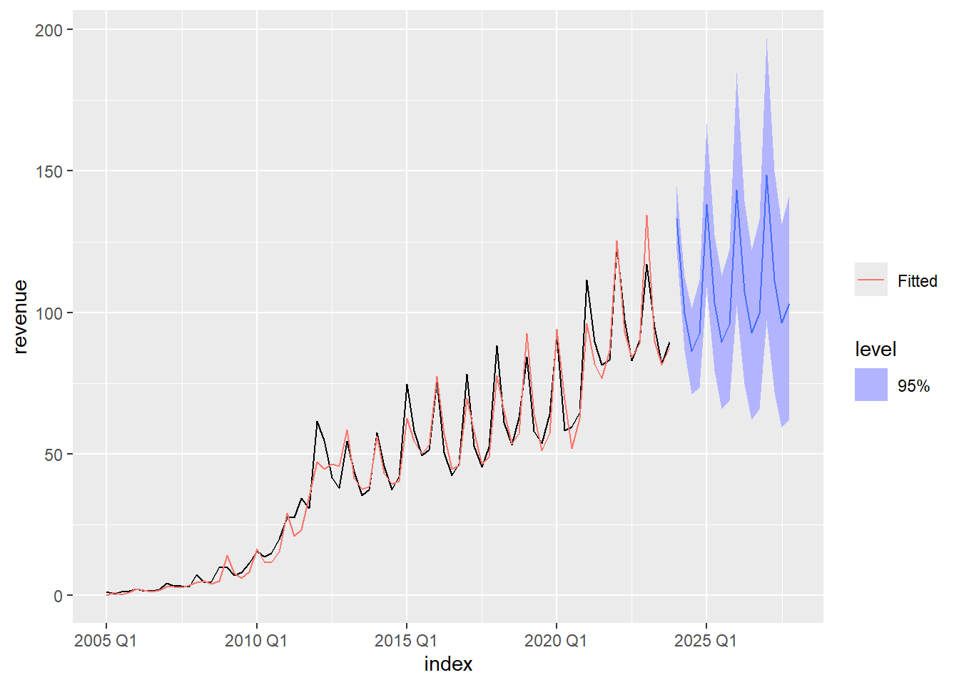
Homework Preview (5 min)
- Review upcoming homework assignment
- Clarify questions
References
- C. C. Holt (1957) Forecasting seasonals and trends by exponentially weighted moving averages, ONR Research Memorandum, Carnegie Institute of Technology 52. (Reprint at https://doi.org/10.1016/j.ijforecast.2003.09.015).
- P. R. Winters (1960). Forecasting sales by exponentially weighted moving averages. Management Science, 6, 324–342. (Reprint at https://doi.org/10.1287/mnsc.6.3.324.)