Covariance and Correlation

Chapter 2: Lesson 1

Learning Outcomes

Compute the key statistics used to describe the linear relationship between two variables

• Compute the sample mean
• Compute the sample variance
• Compute the sample standard deviation
• Compute the sample covariance
• Compute the sample correlation coefficient
• Explain sample covariance using a scatter plot

Interpret the key statistics used to describe sample data

• Interpret the sample mean
• Interpret the sample variance
• Interpret the sample standard deviation
• Interpret the sample covariance
• Interpret the sample correlation coefficient

Preparation

• Read Sections 2.1-2.2.2 and 2.2.4

Learning Journal Exchange (10 min)

• Review another student’s journal
• What would you add to your learning journal after reading your partner’s?
• What would you recommend your partner add to their learning journal?
• Sign the Learning Journal review sheet for your peer

Class Activity: Variance and Standard Deviation (10 min)

We will explore the variance and standard deviation in this section.

Check Your Understanding

• What do the standard deviation and the variance measure?

The following code simulates observations of a random variable. We will use these data to explore the variance and standard deviation.

# Set random seed
set.seed(2412)

# Specify means and standard deviation
n <- 5        # number of points
mu <- 10      # mean
sigma <- 3    # standard deviation

# Simulate normal data
sim_data <- data.frame(x = round(rnorm(n, mu, sigma), 1)) |> 
  arrange(x)

The data simulated by this process are:

6.9, 7.7, 8.1, 10.8, 13.5

Check Your Understanding

• Find the sample mean of these numbers.
• What are some ways to interpret the mean?

The variance and standard deviation are individual numbers that summarize how far the data are from the mean. We first compute the deviations from the mean, $x-\overline{x}$. This is the directed distance from the mean to each data point.

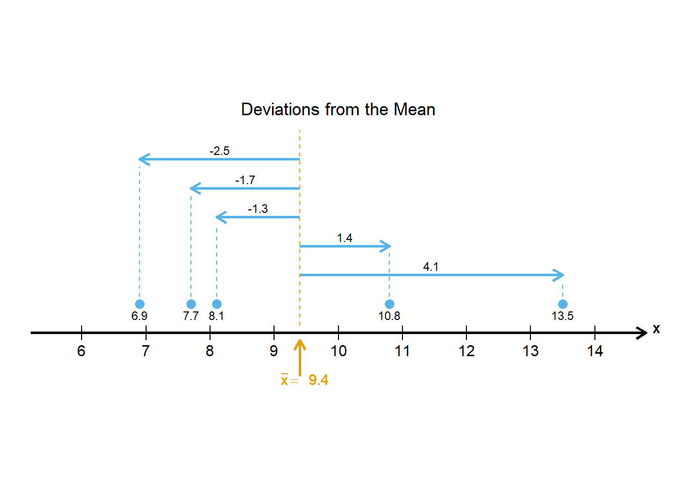
We can summarize this information in a table:

Table 1: Deviations from the mean

$$x_t$$	$$x_t-\overline{x}$$
6.9	-2.5
7.7	-1.7
8.1	-1.3
10.8	1.4
13.5	4.1

Check Your Understanding

How can we obtain one number that summarizes how spread out the data are from the mean? We may try averaging the deviations from the mean.

• What is the average deviation from the mean?
• Will we get the same value with other data sets, or is this just a coincidence?
• What could you do to prevent this from happening?
• Apply your idea. Compute the resulting value that summarizes the spread. What do you get?
• What is the relationship between the sample variance and the sample standard deviation?
• Use a table like the one above to verify that the sample variance is 7.4.
• Show that the sample standard deviation is 2.7203.

Class Activity: Covariance and Correlation (15 min)

Check Your Understanding

• What do you get if you multiply the equations for $r$, $s_x$, and $s_y$ together?

$$r\cdot s_x\cdot s_y=\frac{\sum _{t=1}^n(x-\overline{x})(y-\overline{y})}{\sqrt{\sum _{t=1}^n(x-\overline{x}{)}^2}\sqrt{\sum _{t=1}^n(y-\overline{y}{)}^2}}\cdot \sqrt{\frac{\sum _{t=1}^n(x-\overline{x}{)}^2}{n-1}}\cdot \sqrt{\frac{\sum _{t=1}^n(y-\overline{y}{)}^2}{n-1}}=?$$

Check Your Understanding

• Use the numerical values above to confirm your result. Any discrepancy is due to roundoff error.

Team Activity: Computational Practice (15 min)

Table 3: Computational Practice

Download Excel Handout

Tables-Handout-Excel

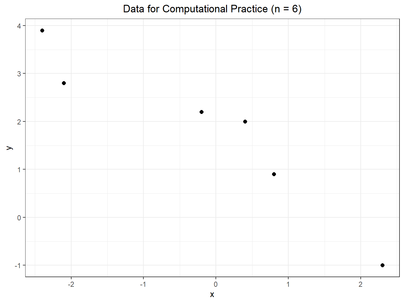
The table below contains values of two time series $\{x_t\}$ and $\{y_t\}$ observed at times $t=1,2,\dots ,6$. We will use these values to practice finding the means, standard deviations, correlation coefficient, and covariance without using built-in R functions.

$$t$$	$$x_t$$	$$y_t$$	$$x_t-\overline{x}$$	$$(x_t-\overline{x}{)}^2$$	$$y_t-\overline{y}$$	$$(y_t-\overline{y}{)}^2$$	$$(x_t-\overline{x})(y_t-\overline{y})$$
1	-2.1	2.8	-1.9	3.61	1	1	-1.9
2	-0.2	2.2
3	0.8	0.9
4	0.4	2
5	2.3	-1
6	-2.4	3.9
sum	-1.2	10.8
$$$$

Use the table above to determine these values:

• $\overline{x}=$

• $\overline{y}=$

• $s_x=$

• $s_y=$

• $r=$

• $cov(x,y)=$

Here is a scatterplot of the data.

Summary

Check Your Understanding

Working with your partner, prepare to explain the following concepts to the class:

• Variance
• Standard deviation
• Correlation
• Covariance

Computations in R (5 min)

Use these commands to load the data from the previous activity into R.

x <- c( -2.1, -0.2, 0.8, 0.4, 2.3, -2.4 )

y <- c( 2.8, 2.2, 0.9, 2, -1, 3.9 )

We can use R to compute the mean, variance, standard deviation, correlation coefficient, and covariance.

Mean, $\overline{x}$

mean(x)

[1] -0.2

Variance, $s_x^2$

var(x)

[1] 3.212

Standard Deviation, $s_x$

sd(x)

[1] 1.792205

Correlation Coefficient, $r$

cor(x, y)

[1] -0.9449384

Covariance, $cov(x,y)$

cov(x, y)

[1] -2.86

Homework Preview (5 min)

• Review upcoming homework assignment
• Clarify questions

Homework

Download Homework

homework_2_1.qmd

Class Activity: Variance and Standard Deviation

Tables-Handout-Excel-key

Solutions to Class Activity: Variance and Standard Deviation

Solution	$$x_t$$	$$x_t-\overline{x}$$	$$(x_t-\overline{x}{)}^2$$
	6.9	-2.5	6.25
	7.7	-1.7	2.89
	8.1	-1.3	1.69
	10.8	1.4	1.96
	13.5	4.1	16.81
Sum	47.0	0.0	29.60

The variance of these values is $s^2=\frac{29.6}{5-1}=3.212$.

The standard deviation is $s=\sqrt{s^2}=\sqrt{3.212}=1.792$.

Team Activity: Computational Practice

Solutions to Team Activity: Computational Practice

Table 3: Computational Practice

$$t$$	$$x_t$$	$$y_t$$	$$x_t-\overline{x}$$	$$(x_t-\overline{x}{)}^2$$	$$y_t-\overline{y}$$	$$(y_t-\overline{y}{)}^2$$	$$(x_t-\overline{x})(y_t-\overline{y})$$
1	-2.1	2.8	-1.9	3.61	1	1	-1.9
2	-0.2	2.2	0	0	0.4	0.16	0
3	0.8	0.9	1	1	-0.9	0.81	-0.9
4	0.4	2	0.6	0.36	0.2	0.04	0.12
5	2.3	-1	2.5	6.25	-2.8	7.84	-7
6	-2.4	3.9	-2.2	4.84	2.1	4.41	-4.62
sum	-1.2	10.8	0	16.06	0	14.26	-14.3

• $\overline{x}=-0.2$

• $\overline{y}=1.8$

• $s_x=1.7922053$

• $s_y=1.6887865$

• $r=-0.9449384$

• $cov(x,y)=-2.86$