Seasonal ARIMA Models

Chapter 7: Lesson 2

Learning Outcomes

Identify seasonal ARIMA models

Define seasonal ARIMA models and their notation (p, d, q)(P, D, Q)[m]
Identify the need for seasonal ARIMA models in time series with seasonal patterns

Apply the fitting procedure for seasonal ARIMA models

Describe the steps involved in fitting seasonal ARIMA models
Determine the appropriate order of differencing (d and D) based on ACF/PACF plots
Select the order of AR and MA terms (p, q, P, Q) using ACF/PACF plots and model selection criteria

Fit seasonal ARIMA models to time series data using R

Use R to fit seasonal ARIMA models
Interpret the output for the ARIMA models, including coefficients and model diagnostics
Forecast future values using the fitted seasonal ARIMA model

Preparation

Read Section 7.3

Learning Journal Exchange (10 min)

Review another student’s journal
What would you add to your learning journal after reading another student’s?
What would you recommend the other student add to their learning journal?
Sign the Learning Journal review sheet for your peer

Definition of Seasonal ARIMA (SARIMA) Models

We can add a seasonal component to an ARIMA model. We call this model a Seasonal ARIMA model, or a SARIMA model. We use differencing at a lag equal to the number of seasons, $s$ . This allows us to remove additional seasonal effects that carry over from one cycle to another.

Recall that if we use a difference of lag 1 to remove a linear trend, we introduce a moving average term. The same thing happens when we introduce a difference with lag $s$ . For the lag $s$ values, we can apply an autoregressive (AR) component at lag $s$ with $P$ parameters, an integrated (I) component with parameter $D$ , and a moving average (MA) component with $Q$ terms. This yields the full SARIMA model.

Definition of SARIMA Models

A Seasonal ARIMA model, or SARIMA model with $s$ seasons can be expressed as:

$Θ_{P} (B^{s}) θ_{p} (B) {(1 - B^{s})}^{D} {(1 - B)}^{d} x_{t} = Φ_{Q} (B^{s}) ϕ_{q} (B) w_{t}$

where

$p$ , $d$ , and $q$ are the parameters for the $A R I M A (p, d, q)$ model applied to the time series and the differences are taken with a lag of 1,
$s$ is the number of seasons, and
$P$ , $D$ , and $Q$ are the parameters for the $A R I M A (P, D, Q)$ model applied to the time series where the differences are taken across a lag of $s$ .

$Θ_{P} (B^{s})$ , $θ_{p} (B)$ , $Φ_{Q} (B^{s})$ , and $ϕ_{q} (B)$ are polynomials of degree $P$ , $p$ , $Q$ , and $q$ , respectively.

We denote this model as $A R I M A (p, d, q) (P, D, Q)_{s}$ or $A R I M A (p, d, q) (P, D, Q) [s]$ .

Looking closely at this model, we can see it is the combination of the ARIMA model $θ_{p} (B) {(1 - B)}^{d} x_{t} = ϕ_{q} (B) w_{t}$ and the same model, after applying a difference across $s$ seasons $Θ_{P} (B^{s}) {(1 - B^{s})}^{D} x_{t} = Φ_{Q} (B^{s}) w_{t}$

Special Cases of a Seasonal ARIMA Model

Stationary SARIMA Models

Stationarity of SARIMA Models

The SARIMA model is, in general, non-stationary. However, there is a special case in which it is stationary. An $A R I M A (p, d, q) (P, D, Q)_{s}$ will be stationary if the following conditions are satisfied:

If $D = d = 0$ , and
The roots of the characteristic equation $Θ_{P} (B^{s}) θ_{p} (B) = 0$ are all greter than 1 in absolute value.

A Simple AR Model with a Seasonal Period of $s$ Units

$A R I M A (0, 0, 0) (1, 0, 0)_{s}$ is given as

$x_{t} = α x_{t - s} + w_{t}$ This model would be appropriate for data where there are $s$ seasons and the value in the season exactly one cycle prior affects the current value. This model is stationary when $| α^{1 / s} | > 1$ .

Stochastic Trends with Seasonal Influences

Many time series with stochastic trends also have seasonal influences. We can extend the previous model as:

$x_{t} = x_{t - 1} + α x_{t - s} - α x_{t - (s + 1)} + w_{t}$

This is equivalent to $\underset{Θ_{1} (B^{12})}{\underset{⏟}{(1 - α B^{12})}} (1 - B) x_{t} = w_{t}$

which is $A R I M A (0, 1, 0) (1, 0, 0)_{s}$ .

Note that we could have written this model as: $\nabla x_{t} = α \nabla x_{t - s} + w_{t}$

This makes it clear that under this model, the change at time $t$ depends on the change at the corresponding time in the previous cycle.

Note that $(1 - B)$ is a factor in the characteristic polynomial, so this model will be non-stationary.

Simple Quarterly Seasonal Moving Average Model (with no Trend)

We can write a simple quarterly seasonal moving average model as

$x_{t} = \underset{(1 - β B^{4}) w_{t}}{\underset{⏟}{w_{t} - β w_{t - 4}}}$

This is an $A R I M A (0, 0, 0) (0, 0, 1)_{4}$ model.

Quarterly Seasonal Moving Average Model with a Stocastic Trend

We can add a stochastic trend to the previous model by including first-order differences:

$x_{t} = x_{t - 1} + w_{t} - β w_{t - 4}$ This is an $A R I M A (0, 1, 0) (0, 0, 1)_{4}$ model.

Quarterly Seasonal Moving Average Model where the Seasonal Terms Contain a Stocastic Trend

We can allow the seasonal components to include a stochastic trend. We apply differencing at the seasonal period. This yields the model

$x_{t} = x_{t - 4} + w_{t} - β w_{t - 4}$

This is an $A R I M A (0, 0, 0) (0, 1, 1)_{4}$ process.

Effects of Differencing

Recall that lag $s$ differencing will remove a linear trend, however if there is a linear trend, differencing at lag 1 will introduce an AR process in the residuals. If a linear model is appropriate in a, say, quarterly series with additive seasonals, then the model could be $x_{t} = a + b t + s_{[t]} + w_{t}$

where $[t]$ is the modulus operator, or $[t]$ is the remainder when $t$ is divided by $4$ . Another way to view this is to note that for a quarterly time series, $[t] = [t - 4]$ .

If we apply first-order differencing at lag 4, we get $\begin{aligned} (1 - B^{4}) x_{t} & = x_{t} - x_{t - 4} \\ = (a + b t + s_{[t]} + w_{t}) - (a + b (t - 4) + s_{[t - 4]} + w_{t - 4}) \\ = (a + b t + s_{[t]} + w_{t}) - (a + b (t - 4) + s_{[t]} + w_{t - 4}) \\ = 4 b + w_{t} - w_{t - 4} \end{aligned}$

This is an $A R I M A (0, 0, 0) (0, 1, 1)_{4}$ process with constant term of $4 b$ .

If we apply first-order differencing at lag 1 and then do the differencing at lag 4, we get the following process: $\begin{aligned} (1 - B^{4}) (1 - B) x_{t} & = (1 - B^{4}) (x_{t} - B x_{t}) \\ = (1 - B^{4}) [(a + b t + s_{[t]} + w_{t}) - B (a + b t + s_{[t]} + w_{t})] \\ = (1 - B^{4}) [(a + b t + s_{[t]} + w_{t}) - (a + b (t - 1) + s_{[t - 1]} + w_{t - 1})] \\ = (1 - B^{4}) [(s_{[t]} + w_{t}) - (- b + s_{[t - 1]} + w_{t - 1})] \\ = (1 - B^{4}) (b + s_{[t]} - s_{[t - 1]} + w_{t} - w_{t - 1}) \\ = (b + s_{[t]} - s_{[t - 1]} + w_{t} - w_{t - 1}) - B^{4} (b + s_{[t]} - s_{[t - 1]} + w_{t} - w_{t - 1}) \\ = (b + s_{[t]} - s_{[t - 1]} + w_{t} - w_{t - 1}) - (b + s_{[t - 4]} - s_{[t - 5]} + w_{t - 4} - w_{t - 5}) \\ = (s_{[t]} - s_{[t - 1]} + w_{t} - w_{t - 1}) - (s_{[t]} - s_{[t - 1]} + w_{t - 4} - w_{t - 5}) \\ = w_{t} - w_{t - 1} - w_{t - 4} + w_{t - 5} \end{aligned}$

This represents an $A R I M A (0, 1, 1) (0, 1, 1)_{4}$ process without a constant term.

Class Activity: Seasonal ARIMA Models - Retail: General Merchandise Stores (10 min)

Show the code

# Read in retail sales data for "Full-Service Restaurants"
retail_ts <- rio::import("https://byuistats.github.io/timeseries/data/retail_by_business_type.parquet") |>
  filter(naics == 452) |>
  mutate( month = yearmonth(as_date(month)) ) |>
  na.omit() |>
  as_tsibble(index = month)

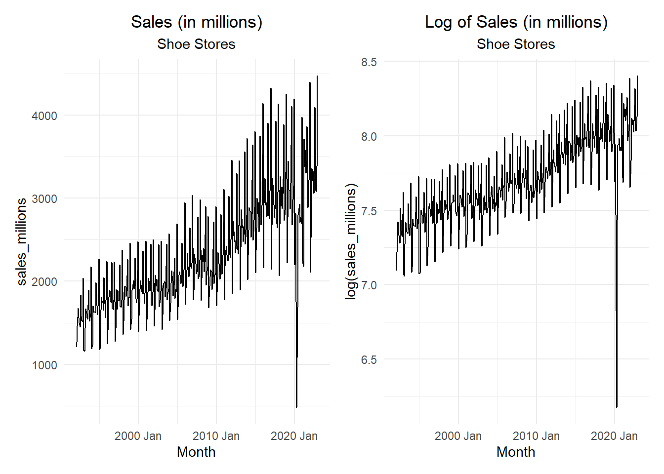
retail_plot_raw <- retail_ts |>
    autoplot(.vars = sales_millions) +
    labs(
      x = "Month",
      y = "sales_millions",
      title = "Sales (in millions)",
      subtitle = "General Merchandise Stores"
    ) +
    theme_minimal() +
    theme(
      plot.title = element_text(hjust = 0.5),
      plot.subtitle = element_text(hjust = 0.5)
    )

retail_plot_log <- retail_ts |>
    autoplot(.vars = log(sales_millions)) +
    labs(
      x = "Month",
      y = "log(sales_millions)",
      title = "Log of Sales (in millions)",
      subtitle = "General Merchandise Stores"
    ) +
    theme_minimal() +
    theme(
      plot.title = element_text(hjust = 0.5),
      plot.subtitle = element_text(hjust = 0.5)
    )

retail_plot_raw | retail_plot_log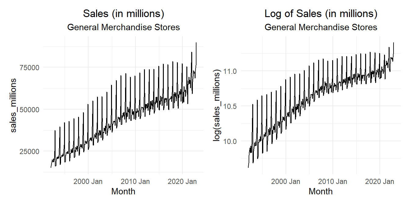

Figure 1: Time plots of the retail sales in General Merchandise stores; time plot of the timt series (left) and the natural logarithm of the time series (right)

Check Your Understanding

Based on the figure above, should the logarithm be applied to the time series? Justify your answer.

Here are a few models we could fit to this time series.

Show the code

retail_ts |>
  model(
    ar_model = ARIMA(sales_millions ~ 1 +
      pdq(1, 1, 0) +
      PDQ(1, 0, 0), approximation = TRUE),
    ma_model = ARIMA(sales_millions ~ 1 + 
      pdq(0, 1, 1) +
      PDQ(0, 0, 1), approximation = TRUE),
    arima_102012 = ARIMA(sales_millions ~ 1 + 
      pdq(1, 0, 2) +
      PDQ(0, 1, 2), approximation = TRUE),
    arima_102102 = ARIMA(sales_millions ~ 1 + 
      pdq(1, 0, 2) +
      PDQ(1, 0, 2), approximation = TRUE),
    arima_112112 = ARIMA(sales_millions ~ 1 + 
      pdq(1, 1, 2) +
      PDQ(1, 1, 2), approximation = TRUE),
    arima_012012 = ARIMA(sales_millions ~ 1 + 
      pdq(0, 1, 2) +
      PDQ(0, 1, 2), approximation = TRUE),
    arima_111111 = ARIMA(sales_millions ~ 1 + 
      pdq(1, 1, 1) +
      PDQ(1, 1, 1), approximation = TRUE),
    ) |>
  glance()

.model	sigma2	log_lik	AIC	AICc	BIC
ar_model	1887684	-3227.047	6462.094	6462.204	6477.759
ma_model	15542235	-3605.992	7219.985	7220.094	7235.650
arima_102012	1264061	-3038.772	6091.544	6091.862	6118.747
arima_112112	1272651	-3030.991	6077.982	6078.393	6109.048
arima_012012	1266582	-3031.167	6074.333	6074.572	6097.633
arima_111111	1270495	-3031.753	6075.506	6075.745	6098.806

Here is the model automatically selected by R.

Show the code

best_fit_retail <- retail_ts |>
  model(
    ar_model = ARIMA(sales_millions ~ 1 +
      pdq(0:2, 0:2, 0:2) +
      PDQ(0:2, 0:2, 0:2), approximation = TRUE))

best_fit_retail

# A mable: 1 x 1
                            ar_model
                             <model>
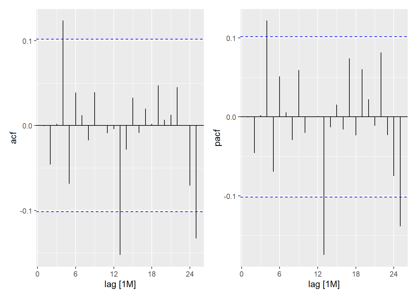
1 <ARIMA(1,0,2)(0,1,2)[12] w/ drift>

This is the acf and pacf of the residuals from the automatically selected model.

Show the code

acf_plot <- best_fit_retail |>
  residuals() |>
  feasts::ACF() |>
  autoplot()

pacf_plot <- best_fit_retail |>
  residuals() |>
  feasts::PACF() |>
  autoplot()

acf_plot | pacf_plot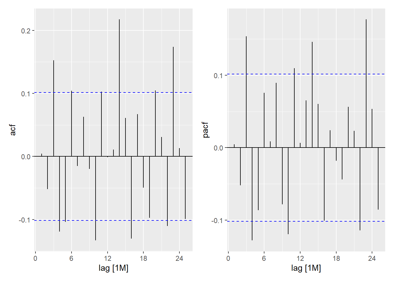

Figure 2: Correlogram (left) and partial correlogram (right) of the residuals from the best-fitting model

Check Your Understanding

What do you notice in the acf and pacf plots?

Here are the coefficients from the automatically-selected model.

Show the code

coefficients(best_fit_retail)

.model	term	estimate	std.error	statistic	p.value
ar_model	ar1	0.9783222	0.0159629	61.287161	0.0000000
ar_model	ma1	-0.8326530	0.0542793	-15.340162	0.0000000
ar_model	ma2	0.1720797	0.0561780	3.063116	0.0023554
ar_model	sma1	-0.4200558	0.0535544	-7.843536	0.0000000
ar_model	sma2	-0.0980853	0.0515993	-1.900905	0.0581129
ar_model	constant	39.3324809	9.4755984	4.150923	0.0000414

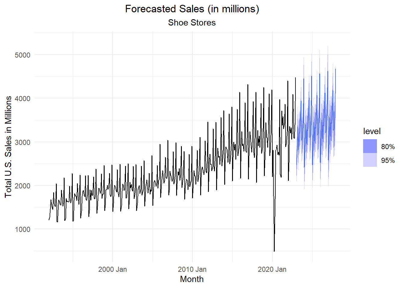
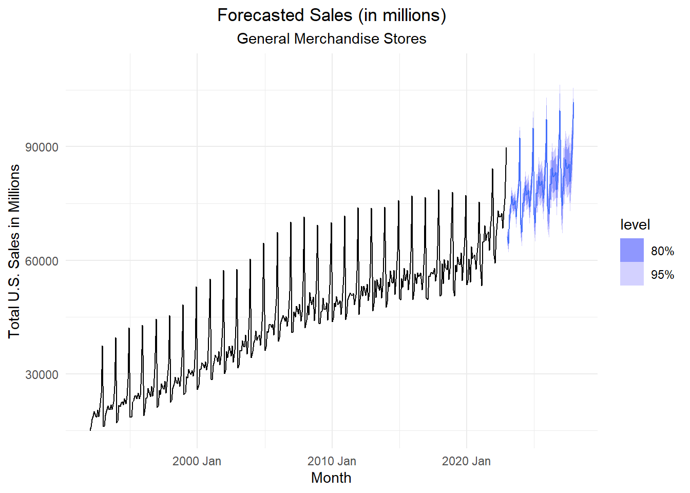
We can forecast future values of this time series using our model.

Show the code

best_fit_retail |>
  forecast(h = "60 months") |>
  autoplot(retail_ts) +
    labs(
      x = "Month",
      y = "Total U.S. Sales in Millions",
      title = "Forecasted Sales (in millions)",
      subtitle = "General Merchandise Stores"
    ) +
    theme_minimal() +
    theme(
      plot.title = element_text(hjust = 0.5),
      plot.subtitle = element_text(hjust = 0.5)
    )

Figure 3: Five-year forecast of the time series based on the best-fitting model

Check Your Understanding

How well does the forecast generated by this model appear to work?

Small-Group Activity: Seasonal ARIMA Models - Retail: Shoe Stores (20 min)

Check Your Understanding

Repeat the analysis above for the retail sales for shoe stores (NAICS code 4482).

Create time plots of the data and the logarithm of the data.
Is it appropriate to take the logarithm of the time series? (Use the appropriate time series for the following.)
Find the best-fitting SARIMA model for the time series.
Determine the model coefficients.
Use the acf and pacf plots of the residuals to assess whether this model adequately models the time series.
Use your model to forecast the value of the time series over the next five years.
How well does the forecast generated by this model appear to work?
Did the downward COVID spike seriously affect the applicability of this model?

Homework Preview (5 min)

Review upcoming homework assignment
Clarify questions

Download Homework

homework_7_2.qmd

Small-Group Activity: Seasonal ARIMA Models - Retail: Shoe Stores

Show the code

# Read in retail sales data for "Full-Service Restaurants"
retail_ts <- rio::import("https://byuistats.github.io/timeseries/data/retail_by_business_type.parquet") |>
  filter(naics == 4482) |>
  mutate( month = yearmonth(as_date(month)) ) |>
  na.omit() |>
  as_tsibble(index = month)

retail_plot_raw <- retail_ts |>
    autoplot(.vars = sales_millions) +
    labs(
      x = "Month",
      y = "sales_millions",
      title = "Sales (in millions)",
      subtitle = "Shoe Stores"
    ) +
    theme_minimal() +
    theme(
      plot.title = element_text(hjust = 0.5),
      plot.subtitle = element_text(hjust = 0.5)
    )

retail_plot_log <- retail_ts |>
    autoplot(.vars = log(sales_millions)) +
    labs(
      x = "Month",
      y = "log(sales_millions)",
      title = "Log of Sales (in millions)",
      subtitle = "Shoe Stores"
    ) +
    theme_minimal() +
    theme(
      plot.title = element_text(hjust = 0.5),
      plot.subtitle = element_text(hjust = 0.5)
    )

retail_plot_raw | retail_plot_log

Show the code

best_fit_retail <- retail_ts |>
  model(
    ar_model = ARIMA(sales_millions ~ 1 +
      pdq(0:2, 0:2, 0:2) +
      PDQ(0:2, 0:2, 0:2), approximation = TRUE))

best_fit_retail

# A mable: 1 x 1
                            ar_model
                             <model>
1 <ARIMA(1,0,2)(0,1,2)[12] w/ drift>

Show the code

acf_plot <- best_fit_retail |>
  residuals() |>
  feasts::ACF() |>
  autoplot()

pacf_plot <- best_fit_retail |>
  residuals() |>
  feasts::PACF() |>
  autoplot()

acf_plot | pacf_plot

Show the code

best_fit_retail |>
  glance()

# A tibble: 1 × 8
  .model   sigma2 log_lik   AIC  AICc   BIC ar_roots  ma_roots  
  <chr>     <dbl>   <dbl> <dbl> <dbl> <dbl> <list>    <list>    
1 ar_model 36049.  -2401. 4817. 4817. 4844. <cpl [1]> <cpl [26]>

Show the code

coefficients(best_fit_retail)

# A tibble: 6 × 6
  .model   term     estimate std.error statistic  p.value
  <chr>    <chr>       <dbl>     <dbl>     <dbl>    <dbl>
1 ar_model ar1         0.907    0.0423     21.4  2.50e-66
2 ar_model ma1        -0.234    0.0689     -3.39 7.73e- 4
3 ar_model ma2        -0.362    0.0564     -6.42 4.41e-10
4 ar_model sma1       -0.846    0.0650    -13.0  4.95e-32
5 ar_model sma2        0.176    0.0646      2.72 6.84e- 3
6 ar_model constant    5.09     1.37        3.73 2.24e- 4

Show the code

best_fit_retail |>
  forecast(h = "60 months") |>
  autoplot(retail_ts) +
    labs(
      x = "Month",
      y = "Total U.S. Sales in Millions",
      title = "Forecasted Sales (in millions)",
      subtitle = "Shoe Stores"
    ) +
    theme_minimal() +
    theme(
      plot.title = element_text(hjust = 0.5),
      plot.subtitle = element_text(hjust = 0.5)
    )

Learning Outcomes

Preparation

Learning Journal Exchange (10 min)

Definition of Seasonal ARIMA (SARIMA) Models

Special Cases of a Seasonal ARIMA Model

Stationary SARIMA Models

A Simple AR Model with a Seasonal Period of s Units

Stochastic Trends with Seasonal Influences

Simple Quarterly Seasonal Moving Average Model (with no Trend)

Quarterly Seasonal Moving Average Model with a Stocastic Trend

Quarterly Seasonal Moving Average Model where the Seasonal Terms Contain a Stocastic Trend

Class Activity: Seasonal ARIMA Models - Retail: General Merchandise Stores (10 min)

Small-Group Activity: Seasonal ARIMA Models - Retail: Shoe Stores (20 min)

Homework Preview (5 min)

A Simple AR Model with a Seasonal Period of $s$ Units