# Additional packages this lesson
pacman::p_load(PerformanceAnalytics) # skewness()Autoregressive Moving Average (ARMA) Models
Chapter 6: Lesson 2
Learning Outcomes
Define autoregressive moving average (ARMA) models
- Write the equation for an ARMA(p,q) model
- Express an ARMA model in terms of the backward shift operators for the AR and MA components
- State facts about ARMA processes related to stationarity, invertibility, special cases, parsimony, and parameter redundancy
- Use ACF and PACF plots to determine if an AR, MA or ARMA model is appropriate for a time series
Apply an iterative time series modeling process
- Fit a regression model to capture trend and seasonality
- Examine residual diagnostic plots to assess autocorrelation
- Fit an ARMA model to the residuals if needed
- Check the residuals of the ARMA model for white noise
- Forecast the original series by combining the regression and ARMA model forecasts
Preparation
- Read Sections 6.5.1 and 6.6-6.7
Learning Journal Exchange (10 min)
Review another student’s journal
What would you add to your learning journal after reading another student’s?
What would you recommend the other student add to their learning journal?
Sign the Learning Journal review sheet for your peer
Packages
pacman::p_load(
  tidyverse,  # ggplot, mutate(), cleaning...
  tsibble,    # as_tsibble()
  fable,      # model(...), forecast(), tidy(), glance()...
  feasts,     # ACF(), PACF()
  ggtime,     # autoplot() for tsibbles
  patchwork,  # + and / for ggplots
  rio         # import()
)
Class Activity: Introduction to Autoregressive Moving Average (ARMA) Models (10 min)
Autoregressive (AR) Models
In Chapter 4, Lesson 3, we learned the definition of an AR model:
The \(AR(p)\) model can be expressed as: \[ \underbrace{\left( 1 - \alpha_1 \mathbf{B} - \alpha_2 \mathbf{B}^2 - \cdots - \alpha_p \mathbf{B}^p \right)}_{\theta_p \left( \mathbf{B} \right)} x_t = w_t \]
Moving Average (MA) Models
The definition of an \(MA(q)\) model is:
Written in terms of the backward shift operator, we have \[ x_t = \underbrace{\left( 1 + \beta_1 \mathbf{B} + \beta_2 \mathbf{B}^2 + \beta_3 \mathbf{B}^3 + \cdots + \beta_{q-1} \mathbf{B}^{q-1} + \beta_q \mathbf{B}^{q} \right)}_{\phi_q(\mathbf{B})} w_t \]
Putting the \(AR\) and \(MA\) models together, we get the \(ARMA\) model.
We can write this as: \[ \theta_p \left( \mathbf{B} \right) x_t = \phi_q \left( \mathbf{B} \right) w_t \]
Comparison of AR and MA Models
Analyzing Time Series with a Regular Seasonal Pattern
Here are some steps you can use to guide your work as you analyze time series with a regular seasonal pattern. Even though these are presented linearly, you may find it helpful to iterate between some of the steps as needed.
Class Activity: Model for the Residuals from the Rexburg Weather Model (15 min)
Show the code
weather_df <- rio::import("https://byuistats.github.io/timeseries/data/rexburg_weather_monthly.csv") |>
  mutate(dates = my(date_text)) |>
  filter(dates >= my("1/2008") & dates <= my("12/2023")) |>
  rename(x = avg_daily_high_temp) |>
  mutate(TIME = 1:n()) |>
  mutate(zTIME = (TIME - mean(TIME)) / sd(TIME),
         month_index = month(dates),
         month_index = factor(month_index, levels = 1:12, labels = month.abb)) |>
  as_tsibble(index = TIME)

weather_df |>
  as_tsibble(index = dates) |>
  autoplot(.vars = x) +
  geom_smooth(method = "lm", se = FALSE, color = "#F0E442") +
    labs(
      x = "Month",
      y = "Mean Daily High Temperature (Fahrenheit)",
      title = "Time Plot of Mean Daily Rexburg High Temperature by Month",
      subtitle = paste0("(", format(weather_df$dates %>% head(1), "%b %Y"), endash, format(weather_df$dates %>% tail(1), "%b %Y"), ")")
    ) +
    theme_minimal() +
    theme(
      plot.title = element_text(hjust = 0.5),
      plot.subtitle = element_text(hjust = 0.5)
    )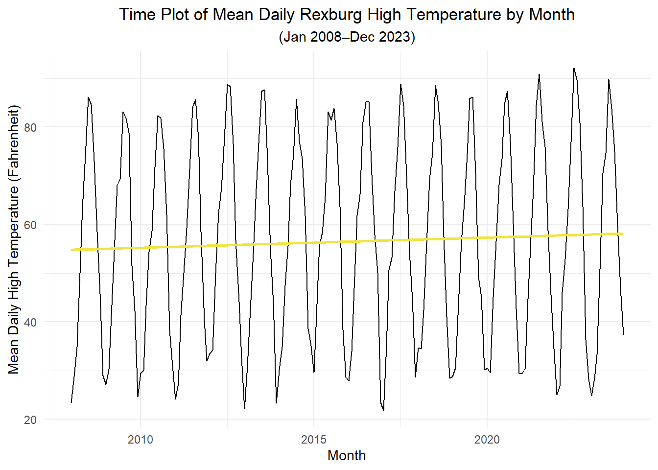
We chose a linear model model.
\[\begin{align*} \log(x_t) &= \beta_0 + \beta_1 \left( \frac{t - \mu_t}{\sigma_t} \right) + s_t + z_t \end{align*}\]
\[\begin{align*} s_t= \begin{cases} \Delta\beta_2 , & t = 2, 14, 26, \ldots ~~~~ ~~(February) \\ \Delta\beta_3 , & t = 2, 14, 26, \ldots ~~~~ ~~(March) \\ ~~~~~~~~⋮ & ~~~~~~~~~~~~⋮ \\ \Delta\beta_{12} , & t = 12, 24, 36, \ldots ~~~~ (December) \end{cases} \end{align*}\]
For convenience, we print the coefficients here.
Show the code
linear_lm <- weather_df |>
  model(linear_5  = TSLM(x ~ zTIME + month_index))

linear_lm |>
  tidy() |>
  mutate(sig = p.value < 0.05)
# A tibble: 13 × 7
.model term estimate std.error statistic p.value sig
<chr> <chr> <dbl> <dbl> <dbl> <dbl> <lgl>
1 linear_5 (Intercept) 27.7 0.953 29.1 1.06e-69 TRUE
2 linear_5 zTIME 0.688 0.276 2.49 1.37e- 2 TRUE
3 linear_5 month_indexFeb 4.18 1.35 3.10 2.24e- 3 TRUE
4 linear_5 month_indexMar 16.7 1.35 12.4 8.51e-26 TRUE
5 linear_5 month_indexApr 27.6 1.35 20.5 8.06e-49 TRUE
6 linear_5 month_indexMay 38.2 1.35 28.3 4.46e-68 TRUE
7 linear_5 month_indexJun 48.3 1.35 35.8 1.47e-83 TRUE
8 linear_5 month_indexJul 58.8 1.35 43.7 2.31e-97 TRUE
9 linear_5 month_indexAug 56.8 1.35 42.2 6.38e-95 TRUE
10 linear_5 month_indexSep 47.3 1.35 35.1 3.57e-82 TRUE
11 linear_5 month_indexOct 30.3 1.35 22.5 4.89e-54 TRUE
12 linear_5 month_indexNov 15.0 1.35 11.1 3.61e-22 TRUE
13 linear_5 month_indexDec 2.03 1.35 1.50 1.35e- 1 FALSEShow the code
r5lin_coef_unrounded <- linear_lm |>
  tidy() |>
  select(term, estimate, std.error)

r5lin_coef <- r5lin_coef_unrounded |>
  round_df(3)

stats_unrounded <- weather_df |>
  as_tibble() |>
  dplyr::select(TIME) |>
  summarize(mean = mean(TIME), sd = sd(TIME))

stats <- stats_unrounded |>
  round_df(3)
The fitted model is:
\[\begin{align*} \log(x_t) &= \beta_0 + 0.688 \left( \frac{t - \mu_t}{\sigma_t} \right) + s_t + z_t \end{align*}\]
\[\begin{align*} s_t= \begin{cases} \Delta\beta_2 , & t = 2, 14, 26, \ldots ~~~~ ~~(February) \\ \Delta\beta_3 , & t = 2, 14, 26, \ldots ~~~~ ~~(March) \\ ~~~~~~~~⋮ & ~~~~~~~~~~~~⋮ \\ \Delta\beta_{12} , & t = 12, 24, 36, \ldots ~~~~ (December) \end{cases} \end{align*}\]
However \(\beta_1\) is for our normalized time variable. If we want to put it in terms of changes each month we would divide our estimate by \(\sigma_t\) (getting an estimate of 0.0124). If we would want it in terms of changes each year we would multiply by 12 (getting an estimate of 0.148).
Show the code
df <- weather_df |>
as_tibble() |>
dplyr::select(TIME, zTIME, month_index) |>
as_tsibble(index = TIME)
linear5_ts <- linear_lm |>
forecast(new_data = df) |>
as_tibble() |>
dplyr::select(TIME, .mean) |>
rename(value = .mean) |>
mutate(Model = "Linear 5")
data_ts <- weather_df |>
as_tibble() |>
rename(value = x) |>
mutate(Model = "Data") |>
dplyr::select(TIME, value, Model)
combined_ts <- bind_rows(data_ts, linear5_ts)
# points only at observed months (integer TIME)
point_ts <- combined_ts |> filter(TIME == floor(TIME))
okabe_ito_colors <- c("#000000", "#E69F00") # Data, Linear 5
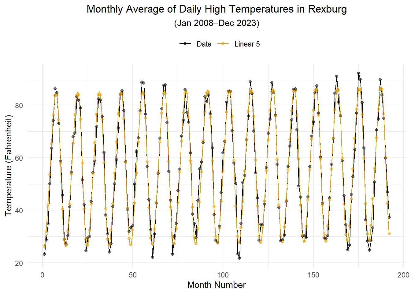
combined_ts |>
ggplot(aes(x = TIME, y = value, color = Model)) +
geom_line() +
geom_point(data = point_ts, alpha = 0.5) +
labs(
x = "Month Number",
y = "Temperature (Fahrenheit)",
title = "Monthly Average of Daily High Temperatures in Rexburg",
subtitle = paste0(
"(",
format(weather_df$dates %>% head(1), "%b %Y"),
endash,
format(weather_df$dates %>% tail(1), "%b %Y"),
")"
)
) +
scale_color_manual(
values = okabe_ito_colors,
name = ""
) +
theme_minimal() +
theme(
plot.title = element_text(hjust = 0.5),
plot.subtitle = element_text(hjust = 0.5),
legend.position = "top",
legend.direction = "horizontal"
)
Fitting an ARMA(p,q) Model
First, we create an acf and pacf plot of the residuals from the model above.
Show the code
linear_lm |>
  residuals() |>
  ACF() |>
  autoplot(var = .resid)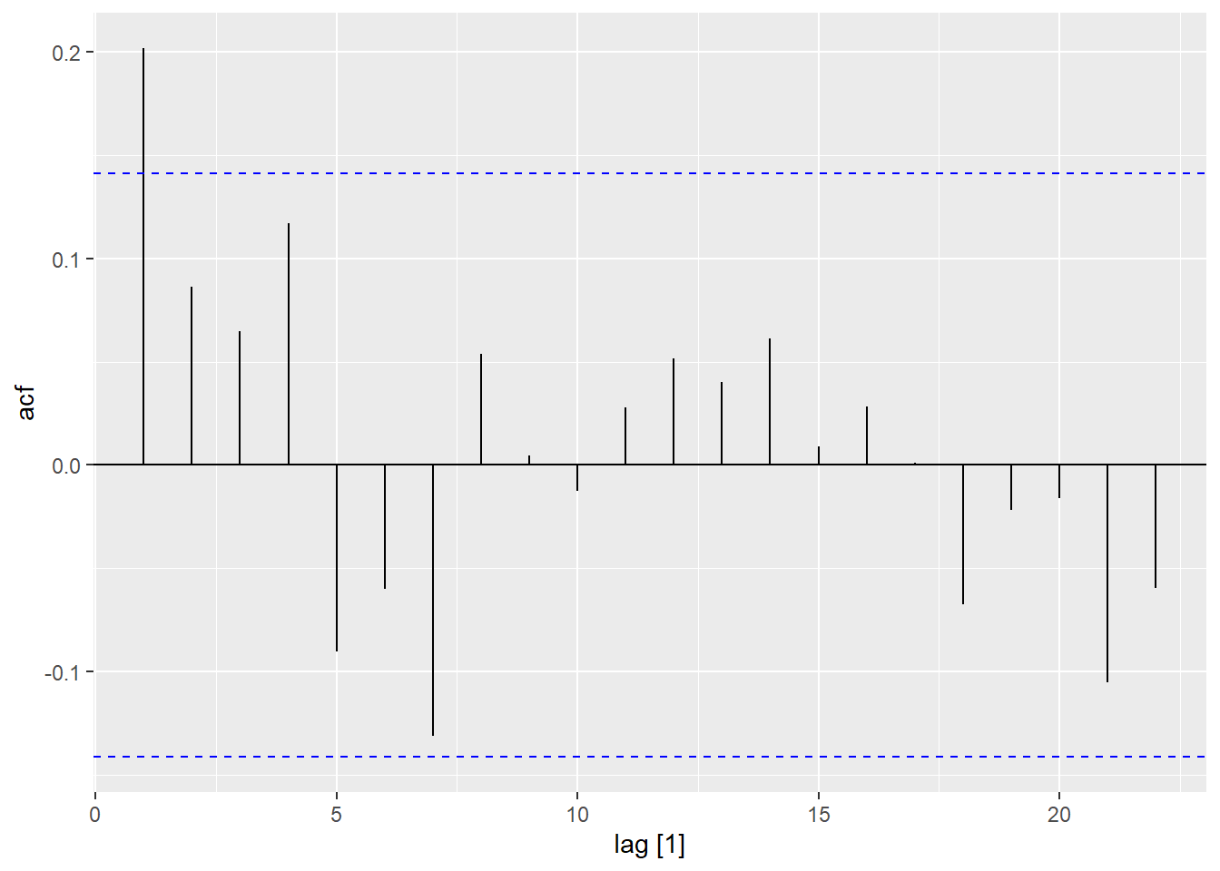
Show the code
linear_lm |>
  residuals() |>
  PACF() |>
  autoplot(var = .resid)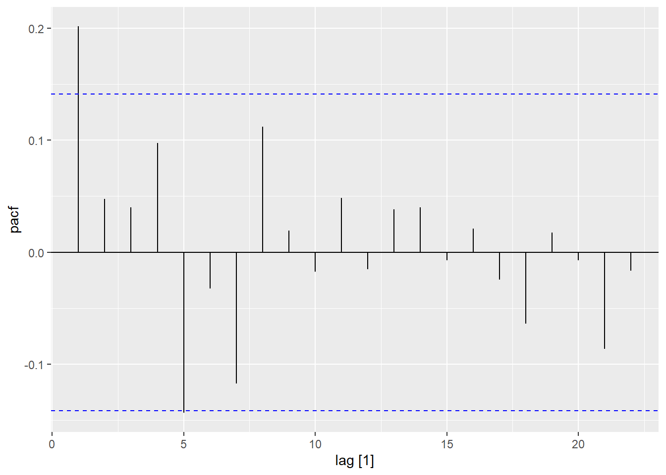
Here are summaries of some ARMA models that could be constructed.
model_resid <- linear_lm |>
  #We are taking the residuals of model 1
  residuals() |>
  select(-.model) |>
  # WE are fitting AR/MA/ARMA models to the residuals
  model(
    auto = ARIMA(.resid ~ 1 + pdq(0:2,0,0:2) + PDQ(0, 0, 0)),
    a000 = ARIMA(.resid ~ 1 + pdq(0,0,0) + PDQ(0, 0, 0)),
    a001 = ARIMA(.resid ~ 1 + pdq(0,0,1) + PDQ(0, 0, 0)),
    a002 = ARIMA(.resid ~ 1 + pdq(0,0,2) + PDQ(0, 0, 0)),
    a100 = ARIMA(.resid ~ 1 + pdq(1,0,0) + PDQ(0, 0, 0)),
    a101 = ARIMA(.resid ~ 1 + pdq(1,0,1) + PDQ(0, 0, 0)),
    a102 = ARIMA(.resid ~ 1 + pdq(1,0,2) + PDQ(0, 0, 0)),
    a200 = ARIMA(.resid ~ 1 + pdq(2,0,0) + PDQ(0, 0, 0)),
    a201 = ARIMA(.resid ~ 1 + pdq(2,0,1) + PDQ(0, 0, 0)),
    a202 = ARIMA(.resid ~ 1 + pdq(2,0,2) + PDQ(0, 0, 0)))

model_resid |>
glance() | Model | AIC | AICc | BIC |
|---|---|---|---|
| auto | **1039.2** | **1039.3** | **1049** |
| a000 | 1049.1 | 1049.1 | 1055.6 |
| a001 | 1040.7 | 1040.8 | 1050.5 |
| a002 | 1041.5 | 1041.7 | 1054.5 |
| a100 | **1039.2** | **1039.3** | **1049** |
| a101 | 1040.4 | 1040.6 | 1053.4 |
| a102 | 1042.3 | 1042.6 | 1058.6 |
| a200 | 1040.6 | 1040.9 | 1053.7 |
| a201 | 1042.3 | 1042.7 | 1058.6 |
| a202 | 1044.3 | 1044.7 | 1063.8 |
Show the code
model_resid |>
  tidy() |>
  filter(.model == "auto")
# A tibble: 2 × 6
.model term estimate std.error statistic p.value
<chr> <chr> <dbl> <dbl> <dbl> <dbl>
1 auto ar1 0.247 0.0704 3.50 0.000572
2 auto constant 0.00407 0.257 0.0158 0.987 Show the code
model_resid |>
  select(auto) |>
  residuals() |>
  ACF() |>
  autoplot(var = .resid)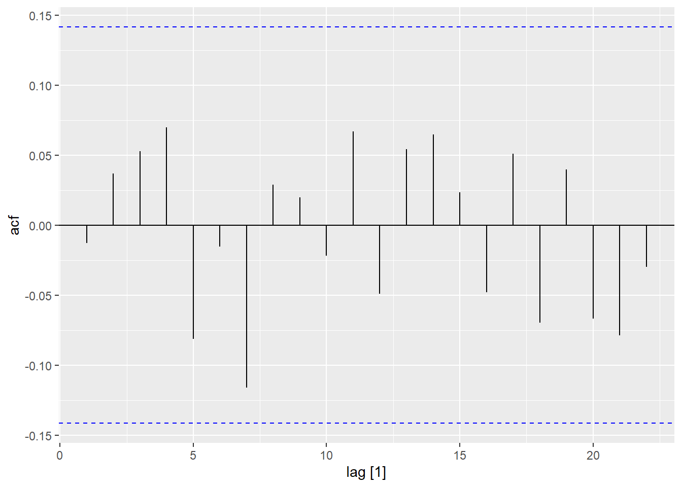
Show the code
model_resid |>
  select(auto) |>
  residuals() |>
  PACF() |>
  autoplot(var = .resid)
Show the code
model_resid |>
  tidy() |>
  filter(.model == "a000")
# A tibble: 1 × 6
.model term estimate std.error statistic p.value
<chr> <chr> <dbl> <dbl> <dbl> <dbl>
1 a000 constant 1.92e-16 0.266 7.24e-16 1.00Show the code
model_resid |>
  select(a000) |>
  residuals() |>
  ACF() |>
  autoplot(var = .resid)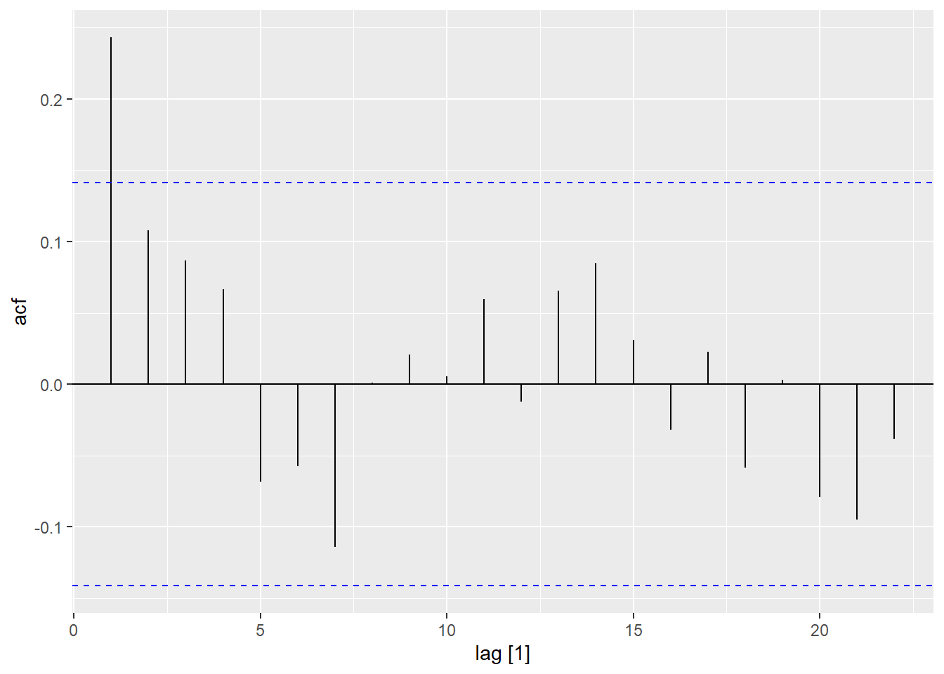
Show the code
model_resid |>
  select(a000) |>
  residuals() |>
  PACF() |>
  autoplot(var = .resid)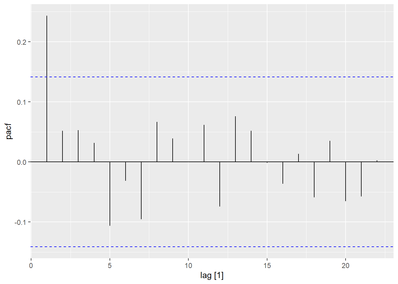
Show the code
model_resid |>
  tidy() |>
  filter(.model == "a001")
# A tibble: 2 × 6
.model term estimate std.error statistic p.value
<chr> <chr> <dbl> <dbl> <dbl> <dbl>
1 a001 ma1 0.219 0.0656 3.34 0.00102
2 a001 constant 0.00283 0.315 0.00900 0.993 Show the code
model_resid |>
  select(a001) |>
  residuals() |>
  ACF() |>
  autoplot(var = .resid)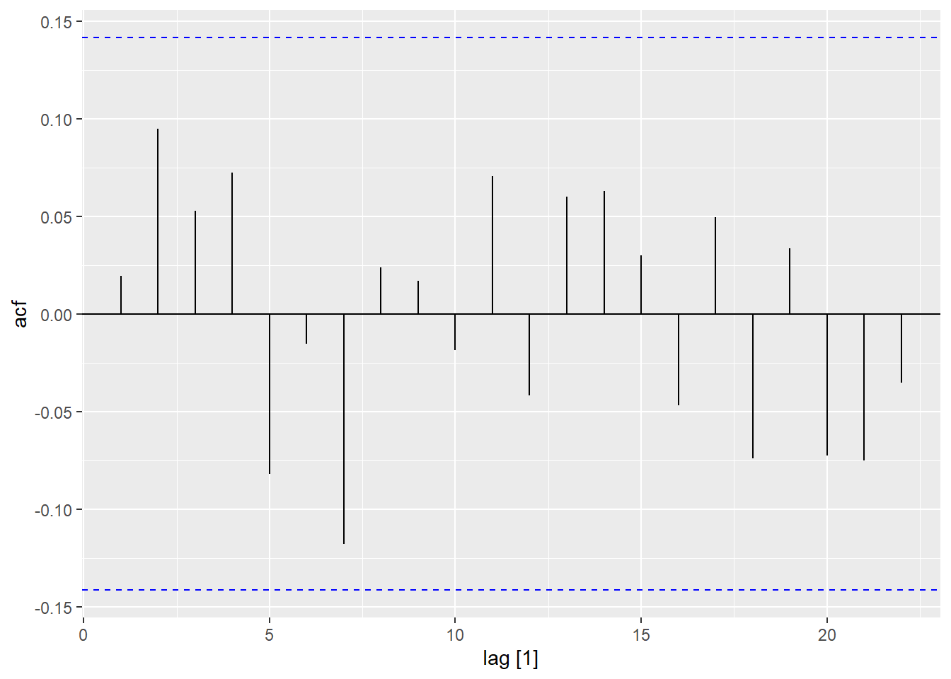
Show the code
model_resid |>
  select(a001) |>
  residuals() |>
  PACF() |>
  autoplot(var = .resid)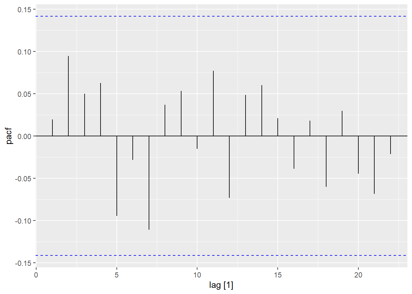
Show the code
model_resid |>
  tidy() |>
  filter(.model == "a002")
# A tibble: 3 × 6
.model term estimate std.error statistic p.value
<chr> <chr> <dbl> <dbl> <dbl> <dbl>
1 a002 ma1 0.230 0.0723 3.18 0.00170
2 a002 ma2 0.0721 0.0653 1.10 0.271
3 a002 constant 0.00562 0.335 0.0168 0.987 Show the code
model_resid |>
  select(a002) |>
  residuals() |>
  ACF() |>
  autoplot(var = .resid)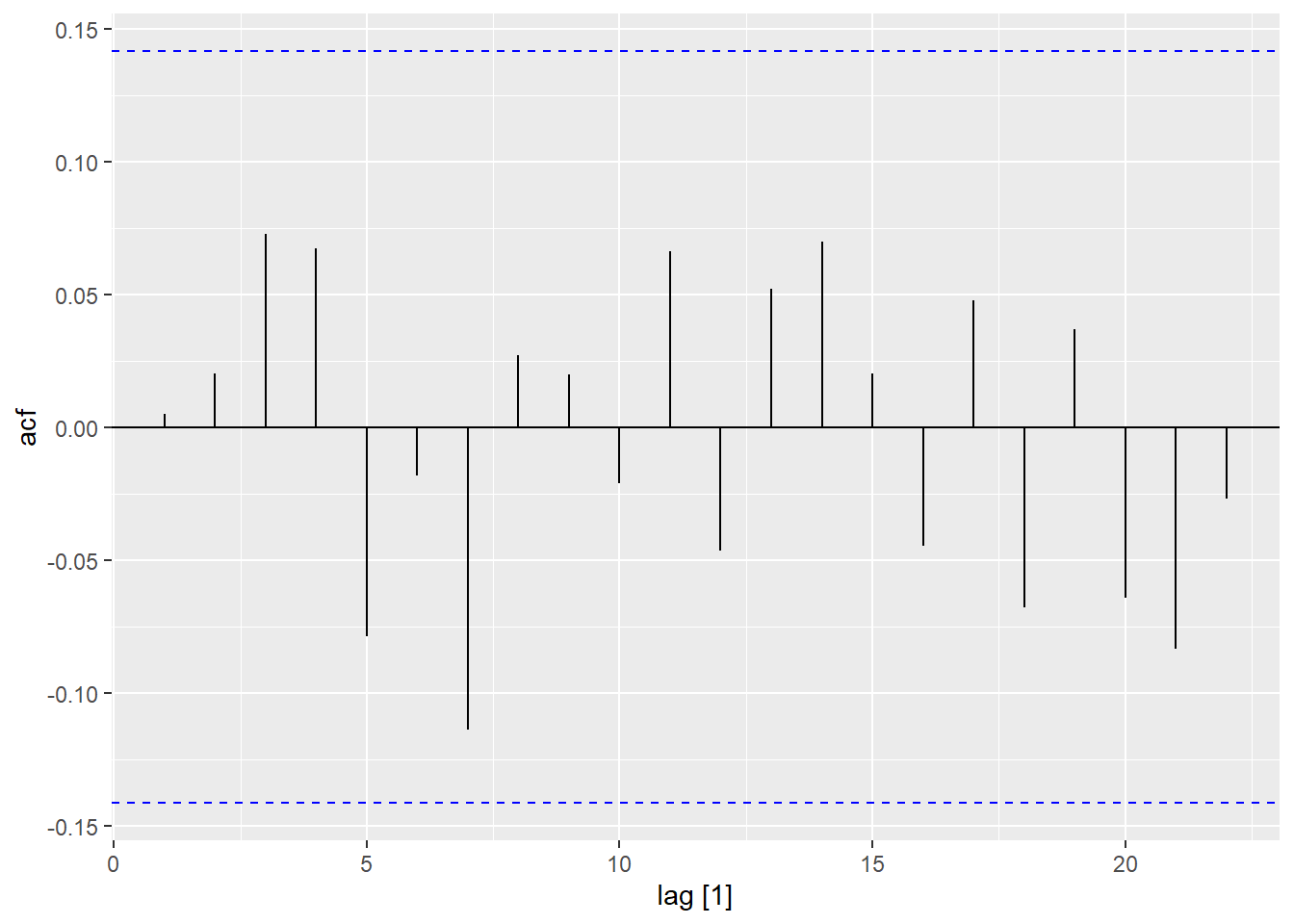
Show the code
model_resid |>
  select(a002) |>
  residuals() |>
  PACF() |>
  autoplot(var = .resid)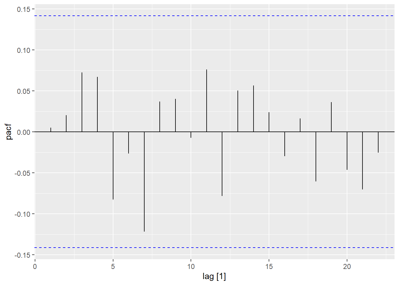
Show the code
model_resid |>
  tidy() |>
  filter(.model == "a100")
# A tibble: 2 × 6
.model term estimate std.error statistic p.value
<chr> <chr> <dbl> <dbl> <dbl> <dbl>
1 a100 ar1 0.247 0.0704 3.50 0.000572
2 a100 constant 0.00407 0.257 0.0158 0.987 Show the code
model_resid |>
  select(a100) |>
  residuals() |>
  ACF() |>
  autoplot(var = .resid)
Show the code
model_resid |>
  select(a100) |>
  residuals() |>
  PACF() |>
  autoplot(var = .resid)
Show the code
model_resid |>
  tidy() |>
  filter(.model == "a101")
# A tibble: 3 × 6
.model term estimate std.error statistic p.value
<chr> <chr> <dbl> <dbl> <dbl> <dbl>
1 a101 ar1 0.511 0.233 2.19 0.0294
2 a101 ma1 -0.283 0.258 -1.10 0.274
3 a101 constant 0.00347 0.183 0.0189 0.985 Show the code
model_resid |>
  select(a101) |>
  residuals() |>
  ACF() |>
  autoplot(var = .resid)
Show the code
model_resid |>
  select(a101) |>
  residuals() |>
  PACF() |>
  autoplot(var = .resid)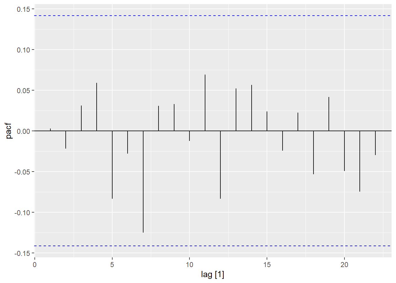
Show the code
model_resid |>
  tidy() |>
  filter(.model == "a102")
# A tibble: 4 × 6
.model term estimate std.error statistic p.value
<chr> <chr> <dbl> <dbl> <dbl> <dbl>
1 a102 ar1 0.549 0.287 1.92 0.0568
2 a102 ma1 -0.317 0.292 -1.09 0.279
3 a102 ma2 -0.0192 0.102 -0.188 0.851
4 a102 constant 0.00323 0.170 0.0190 0.985 Show the code
model_resid |>
  select(a102) |>
  residuals() |>
  ACF() |>
  autoplot(var = .resid)
Show the code
model_resid |>
  select(a102) |>
  residuals() |>
  PACF() |>
  autoplot(var = .resid)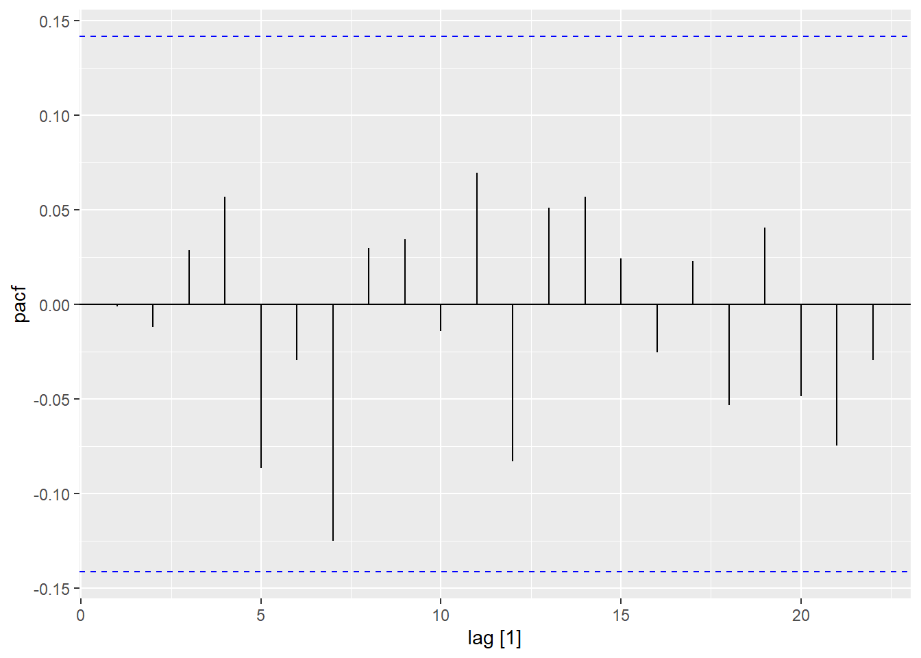
Show the code
model_resid |>
  tidy() |>
  filter(.model == "a200")
# A tibble: 3 × 6
.model term estimate std.error statistic p.value
<chr> <chr> <dbl> <dbl> <dbl> <dbl>
1 a200 ar1 0.234 0.0724 3.23 0.00146
2 a200 ar2 0.0539 0.0724 0.744 0.458
3 a200 constant 0.00506 0.256 0.0197 0.984 Show the code
model_resid |>
  select(a200) |>
  residuals() |>
  ACF() |>
  autoplot(var = .resid)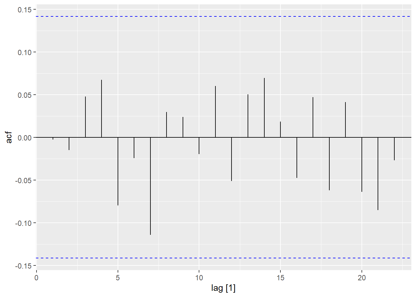
Show the code
model_resid |>
  select(a200) |>
  residuals() |>
  PACF() |>
  autoplot(var = .resid)
Show the code
model_resid |>
  tidy() |>
  filter(.model == "a201")
# A tibble: 4 × 6
.model term estimate std.error statistic p.value
<chr> <chr> <dbl> <dbl> <dbl> <dbl>
1 a201 ar1 0.589 0.478 1.23 0.219
2 a201 ar2 -0.0251 0.148 -0.170 0.865
3 a201 ma1 -0.359 0.471 -0.762 0.447
4 a201 constant 0.00268 0.164 0.0164 0.987Show the code
model_resid |>
  select(a201) |>
  residuals() |>
  ACF() |>
  autoplot(var = .resid)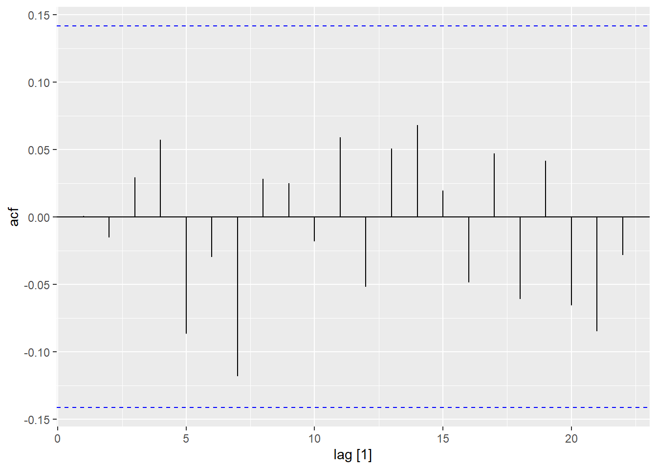
Show the code
model_resid |>
  select(a201) |>
  residuals() |>
  PACF() |>
  autoplot(var = .resid)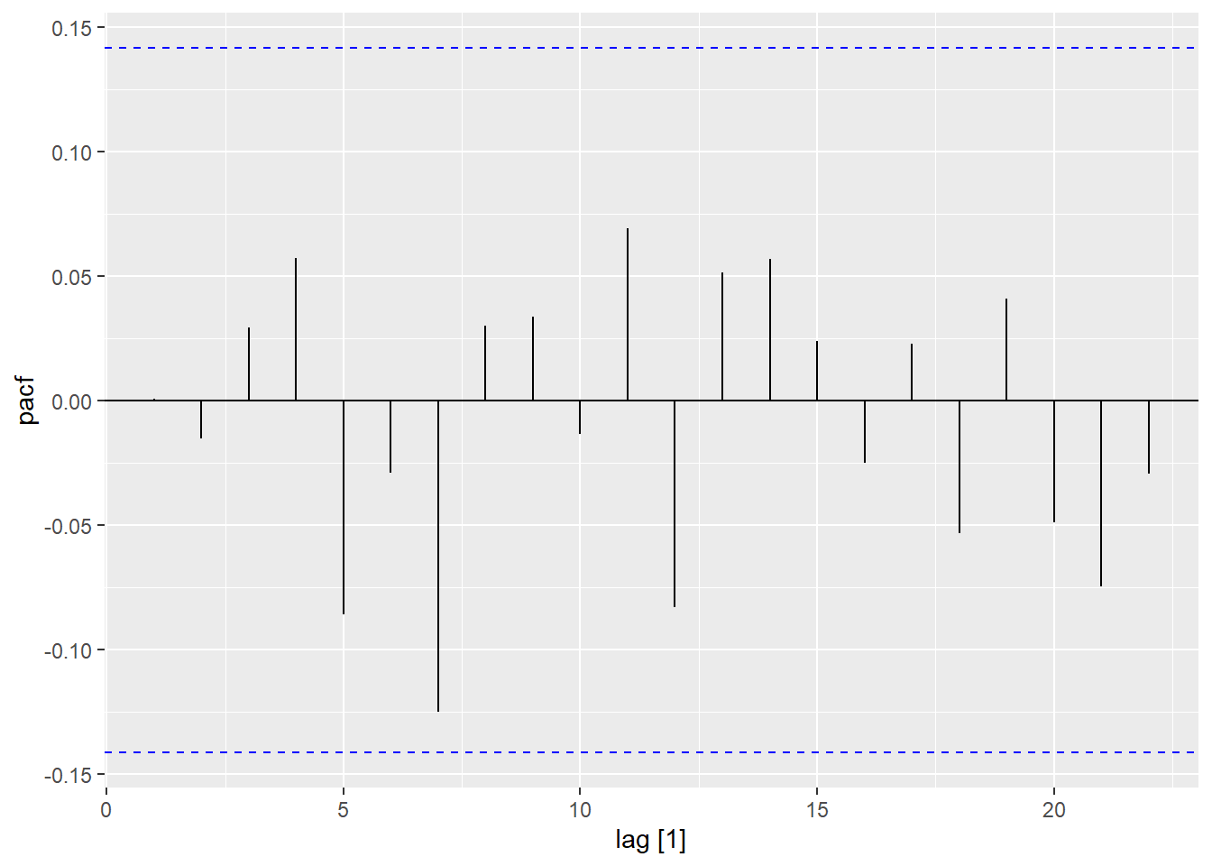
Show the code
model_resid |>
  tidy() |>
  filter(.model == "a202")
# A tibble: 5 × 6
.model term estimate std.error statistic p.value
<chr> <chr> <dbl> <dbl> <dbl> <dbl>
1 a202 ar1 0.305 1.02 0.299 0.765
2 a202 ar2 0.138 0.524 0.264 0.792
3 a202 ma1 -0.0724 1.02 -0.0711 0.943
4 a202 ma2 -0.106 0.316 -0.336 0.737
5 a202 constant 0.00298 0.210 0.0142 0.989Show the code
model_resid |>
  select(a202) |>
  residuals() |>
  ACF() |>
  autoplot(var = .resid)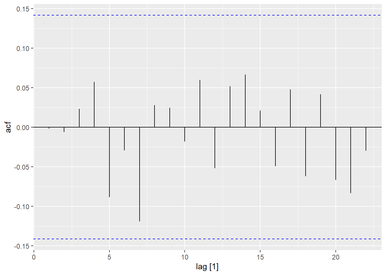
Show the code
model_resid |>
  select(a202) |>
  residuals() |>
  PACF() |>
  autoplot(var = .resid)
Small-Group Activity: Industrial Electricity Consumption in Texas (20 min)
These data represent the amount of electricity used each month for industrial applications in Texas.
Show the code
elec_ts <- rio::import("https://byuistats.github.io/timeseries/data/electricity_tx.csv") |>
  dplyr::select(-comments) |>
  mutate(month = my(month)) |>
  mutate(
    t = 1:n(),
    std_t = (t - mean(t)) / sd(t)
  ) |>
  mutate(month_index = month(month),
    month_index = factor(month_index, levels = 1:12, labels = month.abb)
  ) |>
  as_tsibble(index = month)

elec_plot_raw <- elec_ts |>
    autoplot(.vars = megawatthours) +
    labs(
      x = "Month",
      y = "Megawatt-hours",
      title = "Texas' Industrial Electricity Use"
    ) +
    theme_minimal() +
    theme(
      plot.title = element_text(hjust = 0.5)
    )

elec_plot_log <- elec_ts |>
    autoplot(.vars = log(megawatthours)) +
    labs(
      x = "Month",
      y = "log(Megwatt-hours)",
      title = "Log of Texas' Industrial Electricity Use"
    ) +
    theme_minimal() +
    theme(
      plot.title = element_text(hjust = 0.5)
    )

elec_plot_raw | elec_plot_log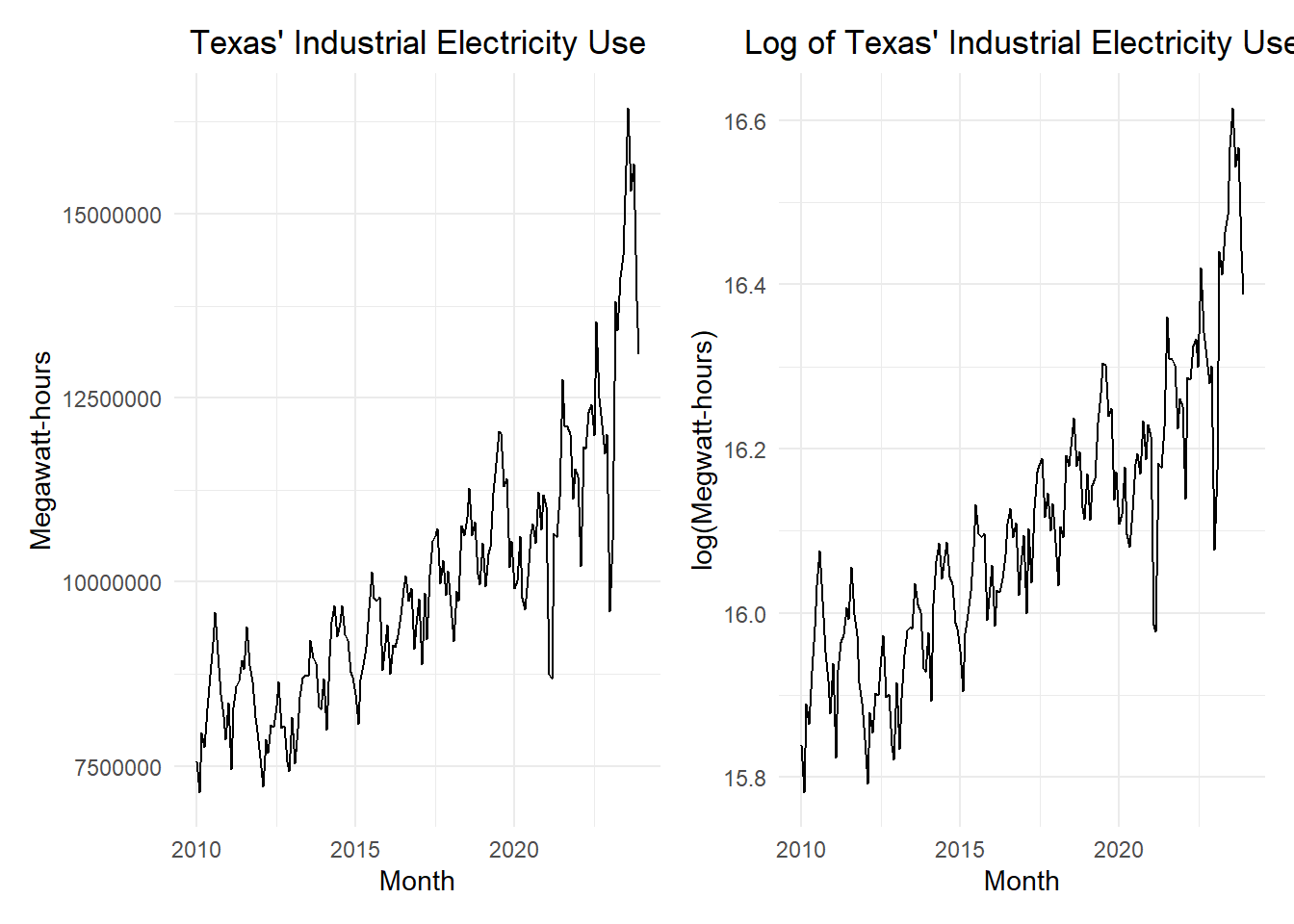
Small Group Activity: Fitting an ARMA(p,q) Model to the Retail Data (30 min)
Apply what you have learned in this lesson to the retail sales data. In particular, consider full-service restaurants (NAICS code 722511).
Here is some code you can use to help you get started.
Show the code
# Read in retail sales data for "Full-Service Restaurants"
retail_ts <- rio::import("https://byuistats.github.io/timeseries/data/retail_by_business_type.parquet") |>
  filter(naics == 722511) |>
  mutate(
    month = yearmonth(as_date(month)),
    month_number = month(month),
    month_index = factor(month_number, levels = 1:12, labels = month.abb)
  ) |>
  mutate(t = 1:n()) |>
  mutate(std_t = (t - mean(t)) / sd(t)) |>
  mutate(
    in_great_recession = ifelse(ym(month) >= my("December 2007") & month <= my("June 2009"), 1, 0),
    after_great_recession = ifelse(ym(month) > my("June 2009"), 1, 0)
  ) |>
  as_tsibble(index = month)

retail_plot_raw <- retail_ts |>
    autoplot(.vars = sales_millions) +
    labs(
      x = "Month",
      y = "sales_millions",
      title = "Other General Merchandise Sales"
    ) +
    theme_minimal() +
    theme(
      plot.title = element_text(hjust = 0.5)
    )

retail_plot_log <- retail_ts |>
    autoplot(.vars = log(sales_millions)) +
    labs(
      x = "Month",
      y = "log(sales_millions)",
      title = "Logarithm of Other Gen. Merch. Sales"
    ) +
    theme_minimal() +
    theme(
      plot.title = element_text(hjust = 0.5)
    )

retail_plot_raw | retail_plot_log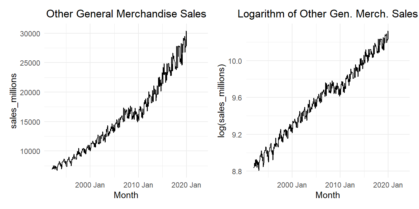
Show the code
retail_final_lm <- retail_ts |>
  model(retail_full = TSLM(log(sales_millions) ~
      (in_great_recession * std_t) + (after_great_recession * std_t)
      + (in_great_recession * I(std_t^2) ) + (after_great_recession * I(std_t^2) )
      + (in_great_recession * I(std_t^3) ) + (after_great_recession * I(std_t^3) )
      + month_index # Note sin6 is omitted
    )
    )

retail_final_lm |>
  tidy() |>
  mutate(sig = p.value < 0.05) |>
  knitr::kable(format = "html", align='ccccccc', escape = FALSE, width = NA, row.names = FALSE) |>
kable_styling(full_width = FALSE, "striped")| .model | term | estimate | std.error | statistic | p.value | sig |
|---|---|---|---|---|---|---|
| retail_full | (Intercept) | 9.6412486 | 0.0078717 | 1224.7969598 | 0.0000000 | TRUE |
| retail_full | in_great_recession | 0.1057700 | 0.1187801 | 0.8904693 | 0.3738957 | FALSE |
| retail_full | std_t | 0.4905760 | 0.0326870 | 15.0083105 | 0.0000000 | TRUE |
| retail_full | after_great_recession | -0.1556298 | 0.0312565 | -4.9791109 | 0.0000011 | TRUE |
| retail_full | I(std_t^2) | -0.0163208 | 0.0458329 | -0.3560935 | 0.7220097 | FALSE |
| retail_full | I(std_t^3) | -0.0102056 | 0.0178717 | -0.5710498 | 0.5683744 | FALSE |
| retail_full | month_indexFeb | -0.0070336 | 0.0069238 | -1.0158589 | 0.3104787 | FALSE |
| retail_full | month_indexMar | 0.0926412 | 0.0069328 | 13.3627121 | 0.0000000 | TRUE |
| retail_full | month_indexApr | 0.0580579 | 0.0069481 | 8.3559455 | 0.0000000 | TRUE |
| retail_full | month_indexMay | 0.1040115 | 0.0069722 | 14.9181309 | 0.0000000 | TRUE |
| retail_full | month_indexJun | 0.0708027 | 0.0070106 | 10.0994433 | 0.0000000 | TRUE |
| retail_full | month_indexJul | 0.0932670 | 0.0069604 | 13.3996338 | 0.0000000 | TRUE |
| retail_full | month_indexAug | 0.0994864 | 0.0069554 | 14.3035106 | 0.0000000 | TRUE |
| retail_full | month_indexSep | 0.0138789 | 0.0069506 | 1.9967907 | 0.0467108 | TRUE |
| retail_full | month_indexOct | 0.0478117 | 0.0069469 | 6.8824479 | 0.0000000 | TRUE |
| retail_full | month_indexNov | 0.0018207 | 0.0069446 | 0.2621772 | 0.7933568 | FALSE |
| retail_full | month_indexDec | 0.0821955 | 0.0069246 | 11.8700290 | 0.0000000 | TRUE |
| retail_full | in_great_recession:std_t | -2.5718611 | 3.0873172 | -0.8330408 | 0.4054549 | FALSE |
| retail_full | std_t:after_great_recession | 0.0198043 | 0.1413695 | 0.1400891 | 0.8886794 | FALSE |
| retail_full | in_great_recession:I(std_t^2) | 14.8230840 | 24.4731229 | 0.6056883 | 0.5451593 | FALSE |
| retail_full | after_great_recession:I(std_t^2) | 0.1215930 | 0.1888445 | 0.6438792 | 0.5201238 | FALSE |
| retail_full | in_great_recession:I(std_t^3) | -35.1756536 | 60.1509944 | -0.5847892 | 0.5591094 | FALSE |
| retail_full | after_great_recession:I(std_t^3) | -0.0653848 | 0.0766366 | -0.8531788 | 0.3942105 | FALSE |
Show the code
retail_resid_df <- retail_final_lm |>
  residuals() |>
  as_tibble() |>
  dplyr::select(.resid) |>
  rename(x = .resid)

retail_resid_df |>
  mutate(density = dnorm(x, mean(retail_resid_df$x), sd(retail_resid_df$x))) |>
  ggplot(aes(x = x)) +
    geom_histogram(aes(y = after_stat(density)),
        color = "white", fill = "#56B4E9", binwidth = 0.02) +
    geom_line(aes(x = x, y = density)) +
    theme_bw() +
    labs(
      x = "Values",
      y = "Frequency",
      title = "Histogram of Residuals"
    ) +
    theme(
      plot.title = element_text(hjust = 0.5)
    )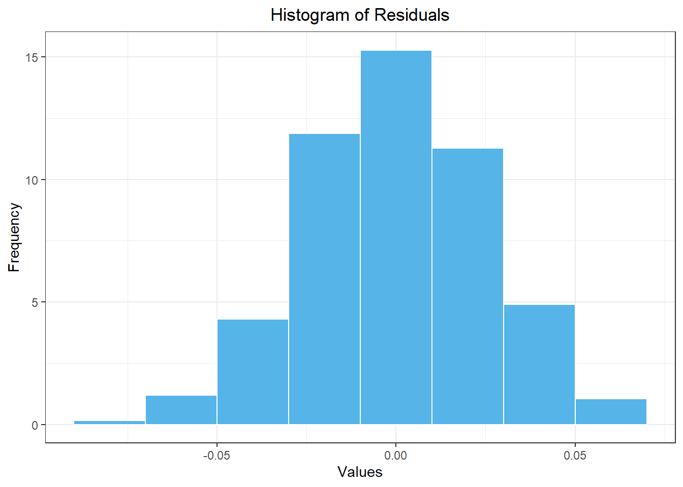
The skewness is given by the command skewness:
Show the code
PerformanceAnalytics::skewness(retail_resid_df$x)[1] 0.01014588Show the code
retail_final_lm |>
  residuals() |>
  ACF() |>
  autoplot(var = .resid)
Show the code
retail_final_lm |>
  residuals() |>
  PACF() |>
  autoplot(var = .resid)
Show the code
################################################################
#   Be sure to adjust this model to match what you did above   #
################################################################
#
# Model without any seasonal trends
retail_no_seasonal_lm <- retail_ts |>
  model(retail_full_quad = TSLM(log(sales_millions) ~
      (in_great_recession * std_t) + (after_great_recession * std_t)
      + (in_great_recession * I(std_t^2) ) + (after_great_recession * I(std_t^2) )
      + (in_great_recession * I(std_t^3) ) + (after_great_recession * I(std_t^3) )
    )
    )

retail_ts |>
  autoplot(.vars = sales_millions) +
  # ggplot(mapping = aes(x = month, y = sales_millions)) +
  # geom_line() +
  geom_line(data = augment(retail_no_seasonal_lm),
            aes(x = month, y = .fitted),
            color = "#E69F00",
            linewidth = 1
            ) +
  geom_line(data = augment(retail_final_lm),
            aes(x = month, y = .fitted),
            color = "blue",
            alpha = 0.7,
            # linewidth = 1
            ) +
  labs(
    x = "Month",
    y = "Sales (Millions of U.S. Dollars)",
    title = paste0(retail_ts$business[1], " (", retail_ts$naics[1], ")")
  ) +
  theme_minimal() +
  theme(plot.title = element_text(hjust = 0.5))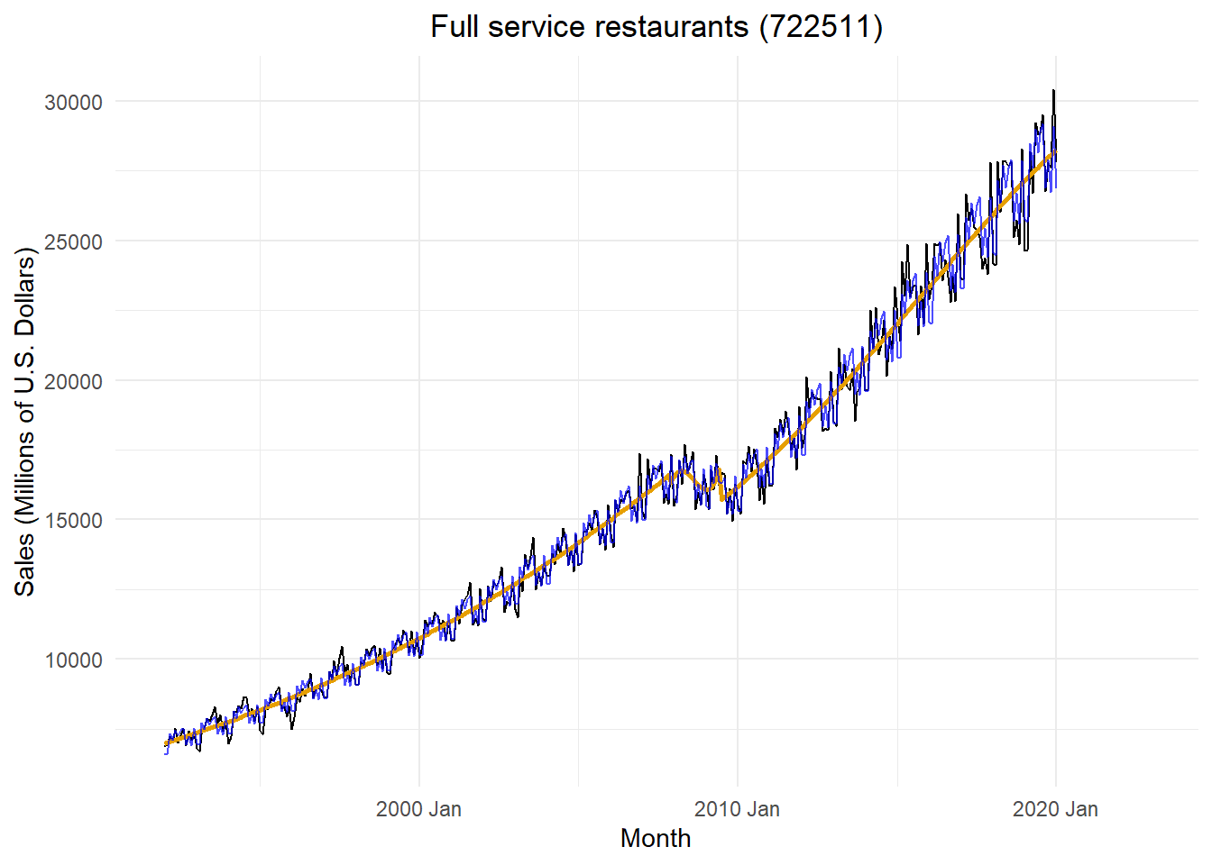
Show the code
model_resid <- retail_final_lm |>
  residuals() |>
  select(-.model) |>
  model(
    auto = ARIMA(.resid ~ 1 + pdq(0:5,0,0:5) + PDQ(0, 0, 0)),
    a000 = ARIMA(.resid ~ 1 + pdq(0,0,0) + PDQ(0, 0, 0)),
    a001 = ARIMA(.resid ~ 1 + pdq(0,0,1) + PDQ(0, 0, 0)),
    a002 = ARIMA(.resid ~ 1 + pdq(0,0,2) + PDQ(0, 0, 0)),
    a003 = ARIMA(.resid ~ 1 + pdq(0,0,3) + PDQ(0, 0, 0)),
    a004 = ARIMA(.resid ~ 1 + pdq(0,0,4) + PDQ(0, 0, 0)),
    a005 = ARIMA(.resid ~ 1 + pdq(0,0,5) + PDQ(0, 0, 0)),
    a100 = ARIMA(.resid ~ 1 + pdq(1,0,0) + PDQ(0, 0, 0)),
    a101 = ARIMA(.resid ~ 1 + pdq(1,0,1) + PDQ(0, 0, 0)),
    a102 = ARIMA(.resid ~ 1 + pdq(1,0,2) + PDQ(0, 0, 0)),
    a103 = ARIMA(.resid ~ 1 + pdq(1,0,3) + PDQ(0, 0, 0)),
    a104 = ARIMA(.resid ~ 1 + pdq(1,0,4) + PDQ(0, 0, 0)),
    a105 = ARIMA(.resid ~ 1 + pdq(1,0,5) + PDQ(0, 0, 0)),
    a200 = ARIMA(.resid ~ 1 + pdq(2,0,0) + PDQ(0, 0, 0)),
    a201 = ARIMA(.resid ~ 1 + pdq(2,0,1) + PDQ(0, 0, 0)),
    a202 = ARIMA(.resid ~ 1 + pdq(2,0,2) + PDQ(0, 0, 0)),
    a203 = ARIMA(.resid ~ 1 + pdq(2,0,3) + PDQ(0, 0, 0)),
    a204 = ARIMA(.resid ~ 1 + pdq(2,0,4) + PDQ(0, 0, 0)),
    a205 = ARIMA(.resid ~ 1 + pdq(2,0,5) + PDQ(0, 0, 0)),
    a300 = ARIMA(.resid ~ 1 + pdq(3,0,0) + PDQ(0, 0, 0)),
    a301 = ARIMA(.resid ~ 1 + pdq(3,0,1) + PDQ(0, 0, 0)),
    a302 = ARIMA(.resid ~ 1 + pdq(3,0,2) + PDQ(0, 0, 0)),
    a303 = ARIMA(.resid ~ 1 + pdq(3,0,3) + PDQ(0, 0, 0)),
    a304 = ARIMA(.resid ~ 1 + pdq(3,0,4) + PDQ(0, 0, 0)),
    a305 = ARIMA(.resid ~ 1 + pdq(3,0,5) + PDQ(0, 0, 0)),
    a400 = ARIMA(.resid ~ 1 + pdq(4,0,0) + PDQ(0, 0, 0)),
    a401 = ARIMA(.resid ~ 1 + pdq(4,0,1) + PDQ(0, 0, 0)),
    a402 = ARIMA(.resid ~ 1 + pdq(4,0,2) + PDQ(0, 0, 0)),
    a403 = ARIMA(.resid ~ 1 + pdq(4,0,3) + PDQ(0, 0, 0)),
    a404 = ARIMA(.resid ~ 1 + pdq(4,0,4) + PDQ(0, 0, 0)),
    a405 = ARIMA(.resid ~ 1 + pdq(4,0,5) + PDQ(0, 0, 0)),
    a500 = ARIMA(.resid ~ 1 + pdq(5,0,0) + PDQ(0, 0, 0)),
    a501 = ARIMA(.resid ~ 1 + pdq(5,0,1) + PDQ(0, 0, 0)),
    a502 = ARIMA(.resid ~ 1 + pdq(5,0,2) + PDQ(0, 0, 0)),
    a503 = ARIMA(.resid ~ 1 + pdq(5,0,3) + PDQ(0, 0, 0)),
    a504 = ARIMA(.resid ~ 1 + pdq(5,0,4) + PDQ(0, 0, 0)),
    a505 = ARIMA(.resid ~ 1 + pdq(5,0,5) + PDQ(0, 0, 0))
  )


# This command indicates which model was selected by "auto"
# model_resid |> select(auto)

model_resid |>
  glance() |>
  # uncomment the next line to only show the "best" models according to these criteria
  # filter(AIC == min(AIC) | AICc == min(AICc) | BIC == min(BIC) | .model == "auto") |>
  knitr::kable(format = "html", align='ccccccc', escape = FALSE, width = NA, row.names = FALSE) |>
kable_styling(full_width = FALSE, "striped")| .model | sigma2 | log_lik | AIC | AICc | BIC | ar_roots | ma_roots |
|---|---|---|---|---|---|---|---|
| auto | 0.0003644 | 841.5138 | -1667.028 | -1666.631 | -1635.677 | -0.5762646+0.8613026i, -0.5762646-0.8613026i, 2.2627735-0.8408307i, 2.2627735+0.8408307i | -0.5154592+0.9948076i, -0.5154592-0.9948076i |
| a000 | 0.0005764 | 762.4127 | -1520.825 | -1520.793 | -1512.988 | ||
| a001 | 0.0004803 | 793.5159 | -1581.032 | -1580.966 | -1569.275 | -2.382155+0i | |
| a002 | 0.0004782 | 794.7146 | -1581.429 | -1581.320 | -1565.754 | -1.822802+2.494324i, -1.822802-2.494324i | |
| a003 | 0.0004109 | 820.4694 | -1630.939 | -1630.775 | -1611.344 | 0.2326238+1.346072e+00i, -1.3798219-1.134128e-17i, 0.2326238-1.346072e+00i | |
| a004 | 0.0004086 | 821.8842 | -1631.768 | -1631.538 | -1608.255 | 0.09044574+1.334121e+00i, -1.28801184-8.558851e-17i, 0.09044574-1.334121e+00i, 4.26337952+0.000000e+00i | |
| a005 | 0.0004097 | 821.8871 | -1629.774 | -1629.466 | -1602.342 | 0.09674194+1.327683e+00i, -1.29555465-1.133215e-16i, 0.09674194-1.327683e+00i, 3.65870427+2.401089e-16i, -19.27340751+4.073186e-17i | |
| a100 | 0.0004615 | 800.2336 | -1594.467 | -1594.402 | -1582.710 | 2.220227+0i | |
| a101 | 0.0004590 | 801.5727 | -1595.145 | -1595.036 | -1579.470 | 1.709493+0i | 6.008737+0i |
| a102 | 0.0004537 | 803.9495 | -1597.899 | -1597.735 | -1578.305 | 2.092518+0i | 0.2913852+2.033057i, 0.2913852-2.033057i |
| a103 | 0.0004091 | 821.6652 | -1631.330 | -1631.100 | -1607.817 | -4.593936+0i | 0.1146925+1.365411e+00i, -1.2737886-9.254356e-17i, 0.1146925-1.365411e+00i |
| a104 | 0.0003923 | 827.7659 | -1641.532 | -1641.224 | -1614.100 | 1.114879+0i | 0.2022091+1.315770e+00i, 0.2022091-1.315770e+00i, 1.0000013-1.396678e-19i, -1.3522966+1.396678e-19i |
| a105 | 0.0003929 | 828.0239 | -1640.048 | -1639.651 | -1608.697 | 1.103023+0i | 1.0000021-3.474159e-21i, -1.3120100+1.688069e-21i, 0.1460054-1.323116e+00i, 0.1460054+1.323116e+00i, 9.3409497+0.000000e+00i |
| a200 | 0.0004586 | 801.7290 | -1595.458 | -1595.349 | -1579.782 | 1.741604-2.524355e-29i, -6.053939+2.524355e-29i | |
| a201 | 0.0004597 | 801.7718 | -1593.544 | -1593.380 | -1573.949 | 1.707303+8.252303e-17i, -8.322029-8.252303e-17i | 17.35635+0i |
| a202 | 0.0004424 | 808.6177 | -1605.235 | -1605.005 | -1581.722 | 1.11252+1.235597i, 1.11252-1.235597i | 0.4783619+1.381186i, 0.4783619-1.381186i |
| a203 | 0.0004020 | 824.8516 | -1635.703 | -1635.395 | -1608.271 | -0.6035275+1.04516i, -0.6035275-1.04516i | -0.3416803+1.043750e+00i, -1.4900939-2.708762e-14i, -0.3416803-1.043750e+00i |
| a204 | 0.0003928 | 828.0543 | -1640.109 | -1639.712 | -1608.757 | 1.103352+5.98217e-21i, -8.074287-5.98217e-21i | 1.0000004+7.183263e-18i, -1.2996070-4.689689e-18i, 0.1403879-1.330860e+00i, 0.1403879+1.330860e+00i |
| a205 | 0.0003944 | 827.7675 | -1637.535 | -1637.038 | -1602.265 | 1.114557-2.019484e-28i, -1.380078+2.019484e-28i | 1.0000002+1.421717e-24i, -1.3049348+6.100457e-23i, 0.2008851-1.317038e+00i, 0.2008851+1.317038e+00i, -1.4390980+0.000000e+00i |
| a300 | 0.0004588 | 802.1164 | -1594.233 | -1594.069 | -1574.638 | 1.561490-1.033976e-24i, -1.559974+3.283859e+00i, -1.559974-3.283859e+00i | |
| a301 | 0.0004395 | 809.7261 | -1607.452 | -1607.222 | -1583.939 | 1.489169-1.620506e-14i, -1.438632+9.829138e-01i, -1.438632-9.829138e-01i | -1.421429+0i |
| a302 | 0.0003535 | 844.0553 | -1674.111 | -1673.803 | -1646.678 | -0.5774684+8.165105e-01i, -0.5774684-8.165105e-01i, 1.7298086-1.440584e-15i | -0.5791562+0.8214559i, -0.5791562-0.8214559i |
| a303 | 0.0003668 | 840.4061 | -1664.812 | -1664.416 | -1633.461 | -0.5727277+8.592709e-01i, -0.5727277-8.592709e-01i, 1.7714851-1.992400e-15i | -0.5205722+9.760787e-01i, -0.5205722-9.760787e-01i, -6.1372611-8.338131e-16i |
| a304 | 0.0003475 | 849.1941 | -1680.388 | -1679.891 | -1645.118 | -0.5791893+0.8188124i, -0.5791893-0.8188124i, 2.5938818+0.0000000i | -0.6126396+0.8363728i, -0.6126396-0.8363728i, -0.2481781-1.7853621i, -0.2481781+1.7853621i |
| a305 | 0.0003467 | 849.2092 | -1678.418 | -1677.809 | -1639.230 | 1.0685657-8.218536e-20i, -0.5815418+8.262367e-01i, -0.5815418-8.262367e-01i | 1.0000002+4.038968e-28i, -0.6708445+8.616210e-01i, -0.6708445-8.616210e-01i, -0.4789424-1.295562e+00i, -0.4789424+1.295562e+00i |
| a400 | 0.0003926 | 828.4866 | -1644.973 | -1644.743 | -1621.460 | 1.0749085+0.6225984i, -0.8155586+1.0088462i, -0.8155586-1.0088462i, 1.0749085-0.6225984i | |
| a401 | 0.0003936 | 828.5076 | -1643.015 | -1642.707 | -1615.583 | 1.079994+0.6285086i, -0.818089+0.9991499i, -0.818089-0.9991499i, 1.079994-0.6285086i | -39.24509+0i |
| a402 | 0.0003644 | 841.5138 | -1667.028 | -1666.631 | -1635.677 | -0.5762646+0.8613026i, -0.5762646-0.8613026i, 2.2627735-0.8408307i, 2.2627735+0.8408307i | -0.5154592+0.9948076i, -0.5154592-0.9948076i |
| a403 | 0.0003546 | 846.4790 | -1674.958 | -1674.461 | -1639.688 | 1.192965+0.5326171i, -0.576099+0.8530305i, -0.576099-0.8530305i, 1.192965-0.5326171i | -0.5438287+0.9807507i, -0.5438287-0.9807507i, 1.5196159+0.0000000i |
| a404 | 0.0003353 | 854.8728 | -1689.746 | -1689.136 | -1650.557 | 1.0047695+0.5596694i, -0.5778036+0.8165460i, -0.5778036-0.8165460i, 1.0047695-0.5596694i | 1.3041509+0.9241362i, -0.5849618+0.8224675i, -0.5849618-0.8224675i, 1.3041509-0.9241362i |
| a405 | 0.0003281 | 859.1436 | -1696.287 | -1695.554 | -1653.179 | 0.8747233+0.5275229i, -0.5781291+0.8169447i, -0.5781291-0.8169447i, 0.8747233-0.5275229i | 0.8829706+6.178753e-01i, -0.5844895+8.272366e-01i, -0.5844895-8.272366e-01i, 0.8829706-6.178753e-01i, -3.5430072+2.343485e-16i |
| a500 | 0.0003936 | 828.5134 | -1643.027 | -1642.719 | -1615.595 | 1.0816019+6.307460e-01i, -0.8181991+9.966800e-01i, -0.8181991-9.966800e-01i, 1.0816019-6.307460e-01i, 30.0866777+1.360548e-16i | |
| a501 | 0.0003943 | 828.6939 | -1641.388 | -1640.991 | -1610.037 | 1.0638793+6.142745e-01i, -0.7829093+1.024026e+00i, -0.7829093-1.024026e+00i, 1.0638793-6.142745e-01i, -1.6336623-1.137029e-16i | -1.791808+0i |
| a502 | 0.0003465 | 849.6644 | -1681.329 | -1680.832 | -1646.059 | 1.3231536+8.089298e-01i, -0.5790055+8.187047e-01i, -0.5790055-8.187047e-01i, 1.3231536-8.089298e-01i, -1.8902606+1.268815e-16i | -0.6099102+0.8427656i, -0.6099102-0.8427656i |
| a503 | 0.0003371 | 853.7754 | -1687.551 | -1686.941 | -1648.362 | 1.1217881+5.589666e-01i, -0.5777105+8.165425e-01i, -0.5777105-8.165425e-01i, 1.1217881-5.589666e-01i, -2.8337480-6.180590e-16i | -0.5852378+8.227538e-01i, -0.5852378-8.227538e-01i, 1.8462959-2.089622e-16i |
| a504 | 0.0003174 | 863.4734 | -1704.947 | -1704.214 | -1661.839 | 0.8683242+5.235238e-01i, -0.5775260+8.164740e-01i, -0.5775260-8.164740e-01i, 0.8683242-5.235238e-01i, 2.5819030-3.684279e-16i | 0.8814018+0.5774635i, -0.5799805+0.8211971i, -0.5799805-0.8211971i, 0.8814018-0.5774635i |
| a505 | 0.0003172 | 864.3520 | -1704.704 | -1703.835 | -1657.677 | 0.8682999+5.163616e-01i, -0.5775959+8.165192e-01i, -0.5775959-8.165192e-01i, 0.8682999-5.163616e-01i, 1.6809996+9.526461e-17i | 0.8968258+5.530958e-01i, -0.5822468+8.218942e-01i, -0.5822468-8.218942e-01i, 0.8968258-5.530958e-01i, 4.7648682+7.447973e-17i |
Show the code
model_resid |>
  select(a504) |>
  residuals() |>
  ACF() |>
  autoplot(var = .resid)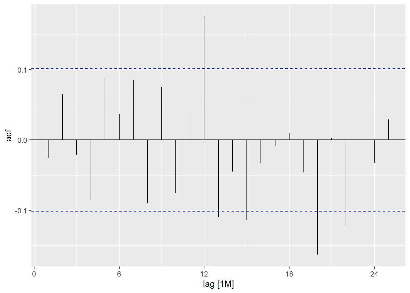
Show the code
model_resid |>
  select(a504) |>
  residuals() |>
  PACF() |>
  autoplot(var = .resid)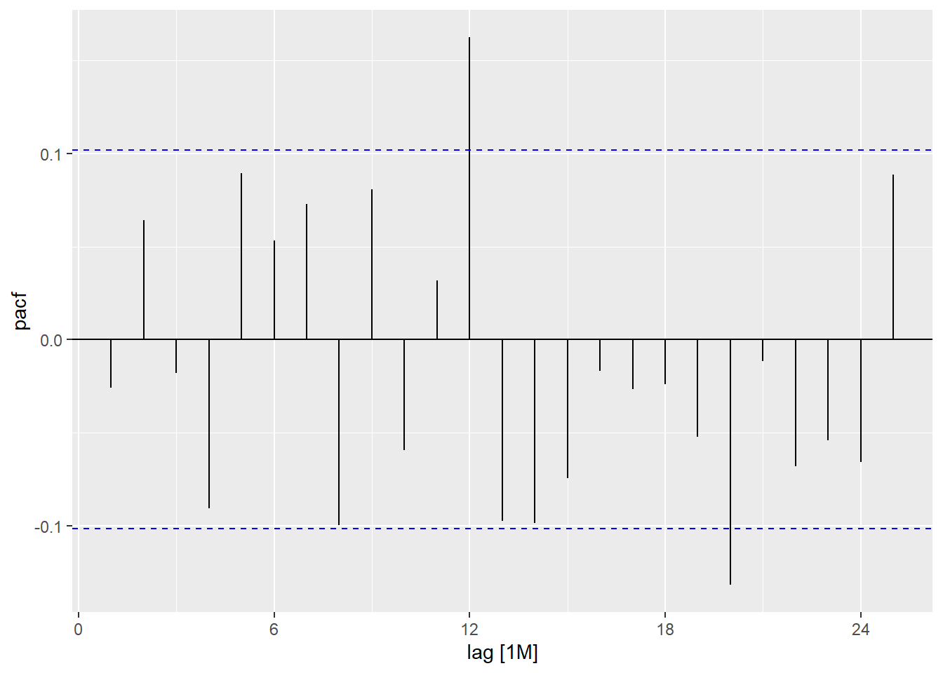
Homework Preview (5 min)
- Review upcoming homework assignment
- Clarify questions