Exponential Smoothing (EWMA)

Chapter 3: Lesson 2

Learning Outcomes

Implement simple exponential smoothing to estimate local mean levels

• Explain forecasting by extrapolation
• State the assumptions of exponential smoothing
• Define exponential weighted moving average (EWMA)
• State the exponential smoothing forecasting equation
• State the EWMA in geometric series form (in terms of x_t only Eq 3.18)
• Explain the EWMA intuitively
• Define the one-step-ahead prediction error (1PE)
• State the SS1PE used to estimate the smoothing parameter of a EWMA
• Indicate when the EWMA smoothing parameter is optimally set as 1/n

Preparation

• Read Section 3.4.1

Learning Journal Exchange (10 min)

• Review another student’s journal

• What would you add to your learning journal after reading another student’s?

• What would you recommend the other student add to their learning journal?

• Sign the Learning Journal review sheet for your peer

Class Discussion: Theory Supporting the EWMA

Our objective is to predict a future value given the first \(n\) observations of a time series. One example would be to forecast sales of an existing product in a stable market.

We assume the following about the time series:

• There is no systematic trend or seasonal effects (or that these have been removed).

• The mean is non-stationary (can change), but we have no idea about the direction.

Check Your Understanding

Match the following definitions to the appropriate term.

1. A future observation of a time series
2. Model assumed in EWMA agorithm
3. Non-stationary mean
4. Random correlated error terms
5. A fixed constant between 0 and 1

1. \(\alpha\)
2. \(\mu_t\)
3. \(w_t\)
4. \(x_{n+k}\)
5. \(x_t = \mu_t + w_t\)

The idea is that we will use past observations to predict future observations. Our best prediction of future observations under this model is the mean of the estimate at the time of the last observation. In symbols, if we want to predict the value of the time series at time \(n+k\), we use our estimate of the time series at time \(n\):

\[ \hat x_{n+k \mid n} = a_n, ~~~~~~~~~~~~~~~~~~\text{where}~~ k = 1, 2, 3, \ldots ~~~~~~~~~~~~~~~~~~~~~~~~~~~~~~~~~~~~~~~~ (3.16) \]

Here are three equivalent expressions that define the EWMA estimation technique:

\[\begin{align} a_t &= \alpha x_t + (1-\alpha) a_{t-1} & (3.15) \\ a_t &= \alpha (x_t - a_{t-1} ) + a_{t-1} & (3.17) \\ a_t &= \alpha x_t + \alpha(1-\alpha) x_{t-1} + \alpha(1-\alpha)^2 x_{t-2} + \alpha(1-\alpha)^3 x_{t-3} + \cdots & (3.18) \end{align}\]

We assume that \(a_1 = x_1\).

Check Your Understanding

• What happens if \(\alpha\) is close to 1?
• What happens if \(\alpha\) is close to 0?
• What is a common “compromise” value for \(\alpha\)?
• Show that Equation (3.15) and (3.17) are equivalent.
• How would you show that Equation (3.18) is equivalent to Equation (3.17)?

Class Activity: Practice Applying the EWMA (20 min)

We will use the following data to practice applying the Exponentially Weighted Moving Average (EWMA) technique. Use \(\alpha = 0.2\).

x <- c( 4.4, 4.2, 4.2, 4, 4.4, 4.7, 4.9, 5.3, 5.4, 5.5 )

Start filling Table 1 by calculating the values of \(a_t\) for each value of \(x_t\).

Table 1: Calculation of \(a_t\) and \(e_t\) for a sample time series

$$t$$	$$x_t$$	$$a_t$$	$$e_t$$
1	4.4
2	4.2
3	4.2
4	4
5	4.4
6	4.7
7	4.9
8	5.3
9	5.4
10	5.5

One-Step-Ahead Prediction Errors

Definition

If we have a time series \(\{x_1, x_2, \ldots, x_n\}\) and start with \(a_1 = x_1\), we can compute the value of \(a_t\) if \(2 \le t \le n\). We define the one-step-ahead prediction error, \(e_t\) as

\[ e_t = x_t - \hat x_{t|t-1} = x_t - a_{t-1} \]

Calculation of \(\alpha\) in R

R uses the one-step-ahead prediction error to estimate \(\alpha\). It chooses \(\alpha\) to minimize

\[ SS1PE = \sum_{t=2}^n e_t^2 = e_2^2 + e_3^2 + e_4^2 + \cdots + e_n^2 \]

where \(a_1 = x_1\).

If the mean of a long time series has not changed much, then this will produce a value of \(\alpha\) that is unduly small. A small value of \(\alpha\) prevents the model from responding to rapid future changes in the time series.

Check Your Understanding

• If the mean of the process does not change much, what is the optimal value of \(\alpha\)?

Computation of the One-Step-Ahead Prediction Errors

Check Your Understanding

• Compute \(e_t\) for the 10 values of \(x\) given in the table above. Add these values to the table.
• Compute SS1PE for these data.

Class Activity: Highway Speeds in New York City (15 min)

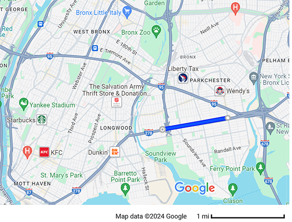
The Bruckner Expressway (I-278) cuts through the Bronx in New York City. Traffic sensors record the speed of cars every 5 minutes between Stratford Avenue and Castle Hill Avenue.

The data from 7/2/2022 through 7/17/2022 are contained in the file ny_speeds.csv. (Source: City of New York Department of Transportation. Online Links: http://a841‐dotweb01.nyc.gov/datafeeds.) These data have been cleaned to align the observations with five minute intervals.

We will read these data into a tsibble.

Figure 1: Google Map showing the location of the data collection.

# Read the ny_speeds data
ny_speeds_dat <- rio::import("https://byuistats.github.io/timeseries/data/ny_speeds.csv")

ny_speeds_tb <- ny_speeds_dat |>
  mutate(
    year = lubridate::year(date),
    month = lubridate::month(date),
    #
    day = lubridate::day(date),
    hour = lubridate::hour(date),
    min = lubridate::minute(date)
  ) |>
  rename(speed = Speed) |>
  dplyr::select(date, year, month, day, hour, min, speed) |>
  tibble()

ny_speeds_ts <- ny_speeds_tb |>
  mutate(index = date) |>
  as_tsibble(index = index)

Here are the first few lines of the tsibble:

# A tsibble: 10 x 8 [5m] <UTC>
   date                 year month   day  hour   min speed index              
   <dttm>              <dbl> <dbl> <int> <int> <int> <dbl> <dttm>             
 1 2022-07-02 00:00:00  2022     7     2     0     0  52.2 2022-07-02 00:00:00
 2 2022-07-02 00:05:00  2022     7     2     0     5  53.4 2022-07-02 00:05:00
 3 2022-07-02 00:10:00  2022     7     2     0    10  55.9 2022-07-02 00:10:00
 4 2022-07-02 00:15:00  2022     7     2     0    15  56.5 2022-07-02 00:15:00
 5 2022-07-02 00:20:00  2022     7     2     0    20  56.5 2022-07-02 00:20:00
 6 2022-07-02 00:25:00  2022     7     2     0    25  53.4 2022-07-02 00:25:00
 7 2022-07-02 00:30:00  2022     7     2     0    30  55.9 2022-07-02 00:30:00
 8 2022-07-02 00:35:00  2022     7     2     0    35  54.7 2022-07-02 00:35:00
 9 2022-07-02 00:40:00  2022     7     2     0    40  53.4 2022-07-02 00:40:00
10 2022-07-02 00:45:00  2022     7     2     0    45  54.0 2022-07-02 00:45:00

Here is a time plot of the data:

autoplot(ny_speeds_ts, .vars = speed) +
  labs(
    x = "Date / Time",
    y = "Traffic Speed (mph)",
    title = "Bruckner Expressway Traffic Speed"
  ) +
  theme(plot.title = element_text(hjust = 0.5))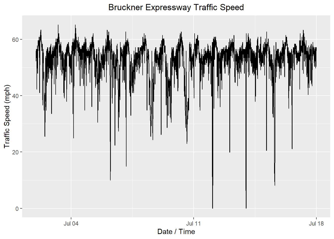

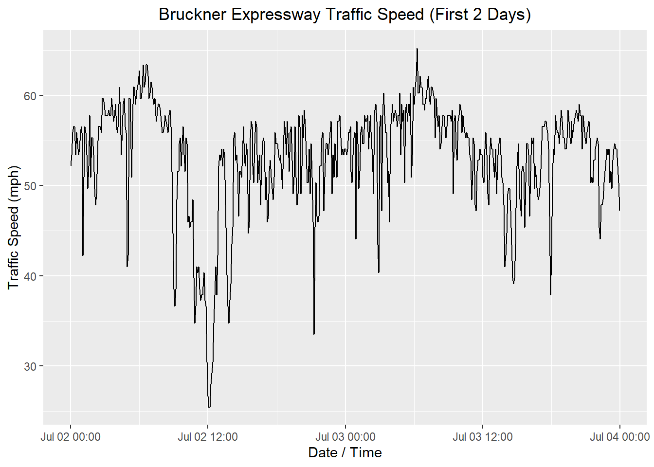
Figure 2: Time series plot of the traffic speed data from July 2 through July 17, 2022

The data set spans 16 days. There is a strong daily pattern, which can be seen by the 16 pairs of peaks and valleys. It might be easier to see if we look at the observations from the first 2 days.

Figure 3: Time series plot of the first two days of the traffic speed data

Check Your Understanding

• What do you no notice about this time series?
• During what parts of the day does the traffic flow tend to be slowest? fastest? What is the reason for this behavior?

Next, we compute the decomposition. We expect that that traffic will fluctuate with daily seasonality. The number of five-minute periods in a day is:

\[ \underbrace{\frac{60}{5}}_{\substack{\text{Number of} \\ \text{5-minute periods} \\ \text{per hour}}} \cdot \underbrace{24}_{\substack{\text{Number of} \\ \text{hours} \\ \text{per day}}} = ~~ 288~~\text{five-minute periods per day} \]

That is, the time series will follow a cycle that repeats every 288 five-minute intervals. Due to the complexity of the time series, we will indicate this to R in our function call. (Try replacing “speed ~ season(288)” in the classical_decomposition command with “speed” and see what happens!)

ny_speeds_decompose <- ny_speeds_ts |>
    model(feasts::classical_decomposition(speed ~ season(288),
        type = "add"))  |>
    components()

autoplot(ny_speeds_decompose)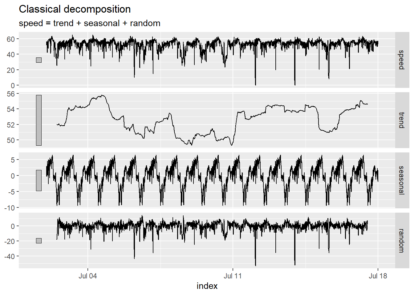

Figure 4: Additive decomposition of the traffic speed time series

Check Your Understanding

• Working with your partner, identify evidence of the daily seasonal component of the speed data.
• How do you explain the sharp downward spikes in the data?
• Does there seem to be a trend in the data? Justify your answer.
• Why is there no estimate for the trend or the random component for the first half of the first day and the last half of the last day?

Here is a plot of the decomposition for the first 4 days of the time series (July 2, 2022 at 0:00 to July 6, 2022 at 0:00).

ny_speeds_decompose |> 
  filter((index) <= mdy_hm("7/6/2022 0:00")) |> 
  autoplot()

Figure 5: Additive decomposition of the first four days of the traffic speed time series

Check Your Understanding

• Consider the seasonal variation. Around what time of day are the speeds highest? When are the speeds lowest?

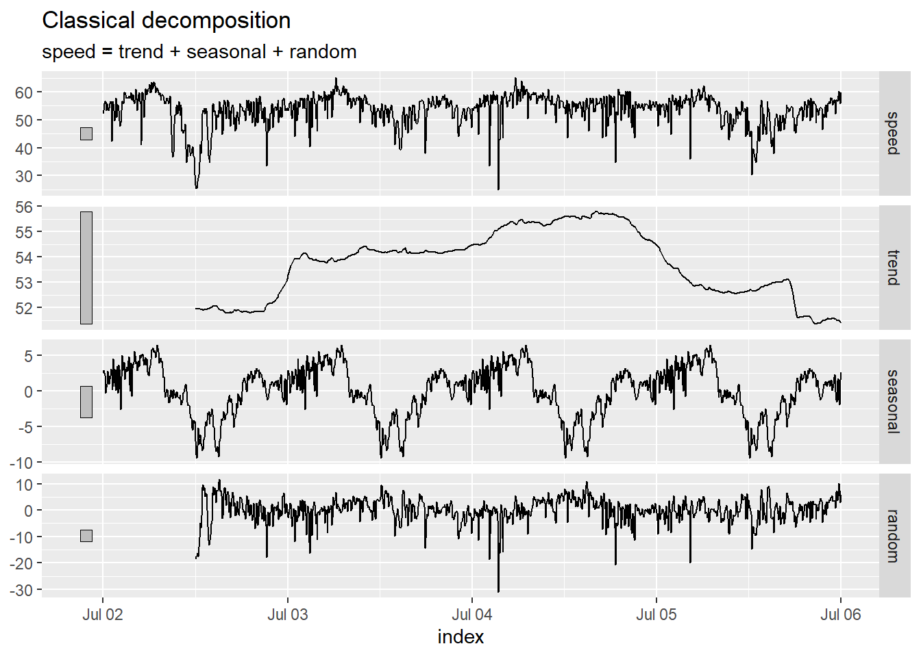
Applying the EWMA when there is a trend and/or seasonal variation

One assumption for the EWMA is that there is no trend or seasonal variation. If present, we need to eliminate the trend and seasonal variation before applying the EWMA algorithm. In this case, we decompose the time series and compute the EWMA for the random component. Finally, we add the trend and seasonal components back in to get the EWMA estimate for the time series.

These data demonstrate distinct seasonal variation. We will need to apply the EWMA algorithm to the random component and later add the seasonal component and trend to our EWMA estimate.

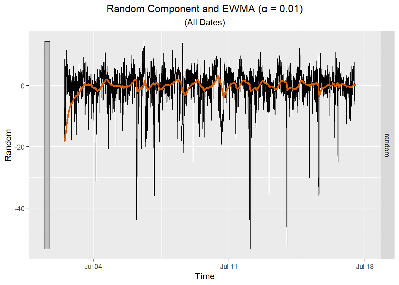
We demonstrate the computation of the EWMA for a few choices of \(\alpha\).

EWMA with \(\alpha = 0.01\)

EWMA

Table 2: Illustration of the computation of the EWMA

Date-Time	Random $$ \hat z_t $$	Computation of $$ a_t $$	$$a_t$$
7/2/2022 12:00	-18.258	-18.258 =	-18.258
7/2/2022 12:05	-17.597	0.01 * (-17.597) + (1 - 0.01) * (-18.258) =	-18.251
7/2/2022 12:10	-17.095	0.01 * (-17.095) + (1 - 0.01) * (-18.251) =	-18.24
7/2/2022 12:15	-16.342	0.01 * (-16.342) + (1 - 0.01) * (-18.24) =	-18.221
7/2/2022 12:20	-17.627	0.01 * (-17.627) + (1 - 0.01) * (-18.221) =	-18.215
7/2/2022 12:25	-14.03	0.01 * (-14.03) + (1 - 0.01) * (-18.215) =	-18.173

Here is a plot showing the EWMA for the random component for all the data.

Figure 6: EWMA superimposed on the random component of the traffic data time series

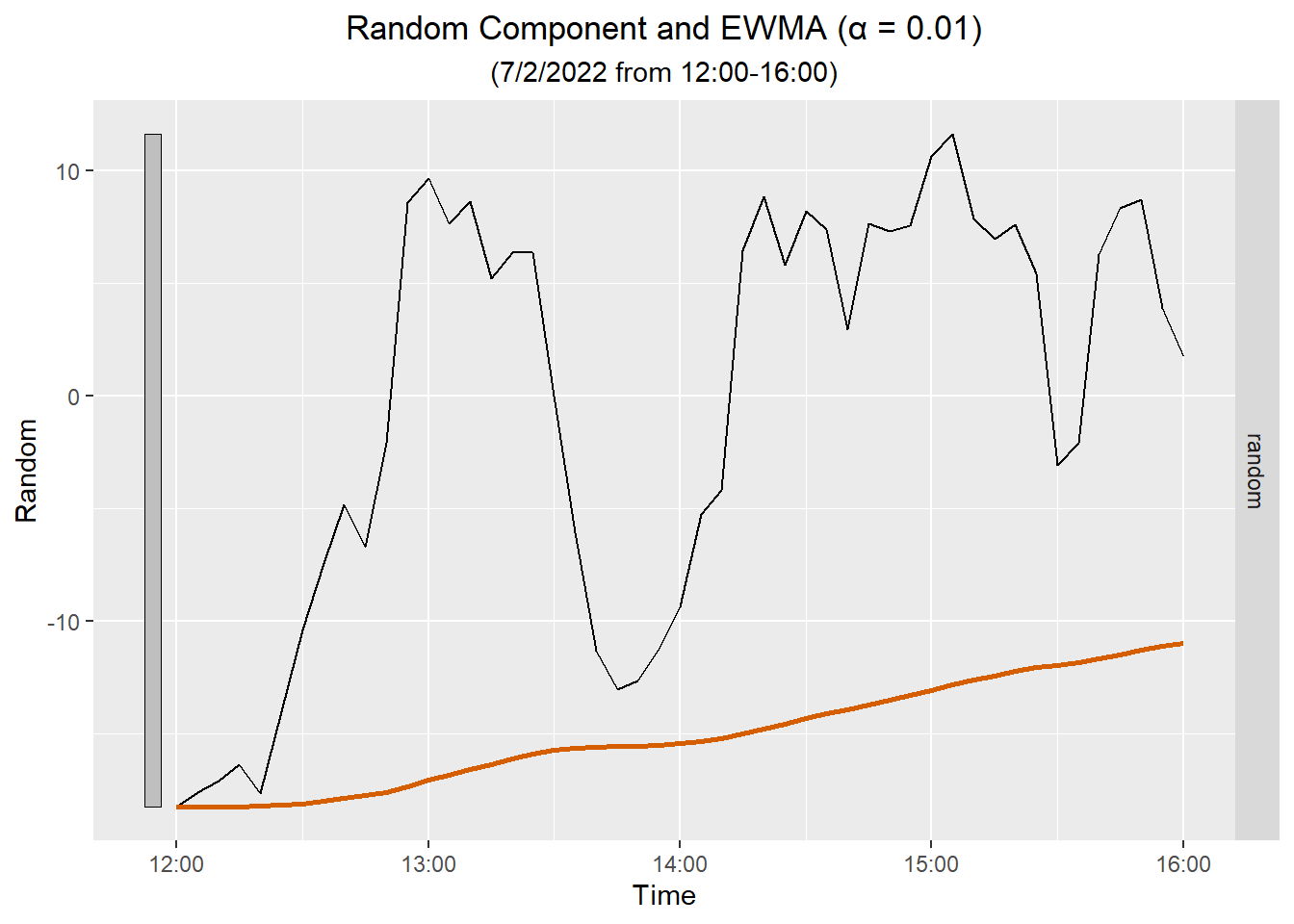
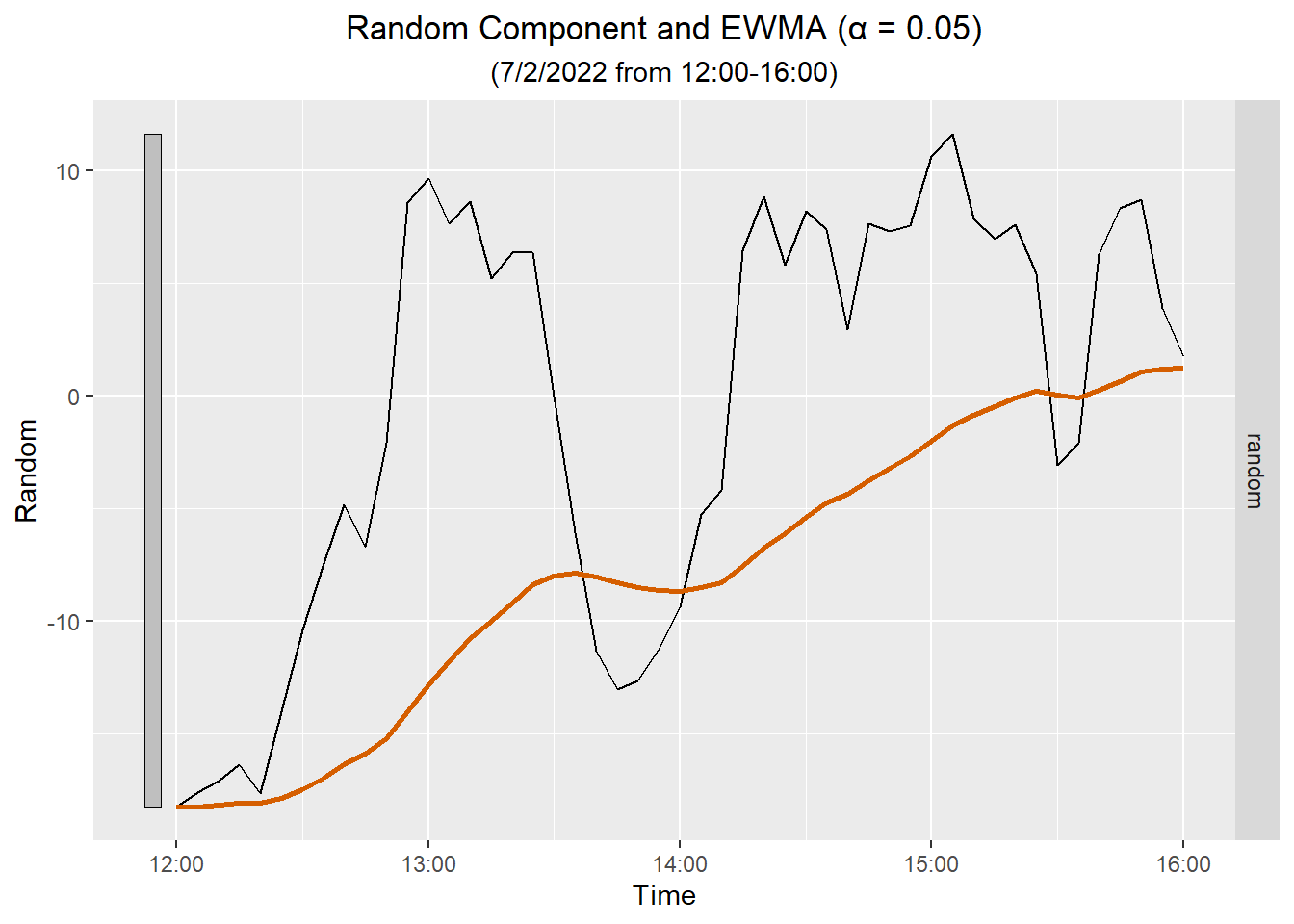
Here is a plot of the EWMA against the random component for four hours:

Figure 7: EWMA superimposed on the random component of the traffic data for a four-hour period

EWMA with \(\alpha = 0.05\)

EWMA

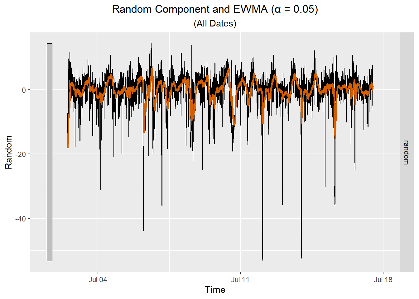
Table 3: Illustration of the computation of the EWMA

Date-Time	Random $$ \hat z_t $$	Computation of $$ a_t $$	$$a_t$$
7/2/2022 12:00	-18.258	-18.258 =	-18.258
7/2/2022 12:05	-17.597	0.05 * (-17.597) + (1 - 0.05) * (-18.258) =	-18.225
7/2/2022 12:10	-17.095	0.05 * (-17.095) + (1 - 0.05) * (-18.225) =	-18.168
7/2/2022 12:15	-16.342	0.05 * (-16.342) + (1 - 0.05) * (-18.168) =	-18.077
7/2/2022 12:20	-17.627	0.05 * (-17.627) + (1 - 0.05) * (-18.077) =	-18.054
7/2/2022 12:25	-14.03	0.05 * (-14.03) + (1 - 0.05) * (-18.054) =	-17.853

Here is a plot showing the EWMA for the random component for all the data.

Figure 8: EWMA superimposed on the random component of the traffic data time series

Here is a plot of the EWMA against the random component for four hours:

Figure 9: EWMA superimposed on the random component of the traffic data for a four-hour period

EWMA with \(\alpha = 0.2\)

EWMA

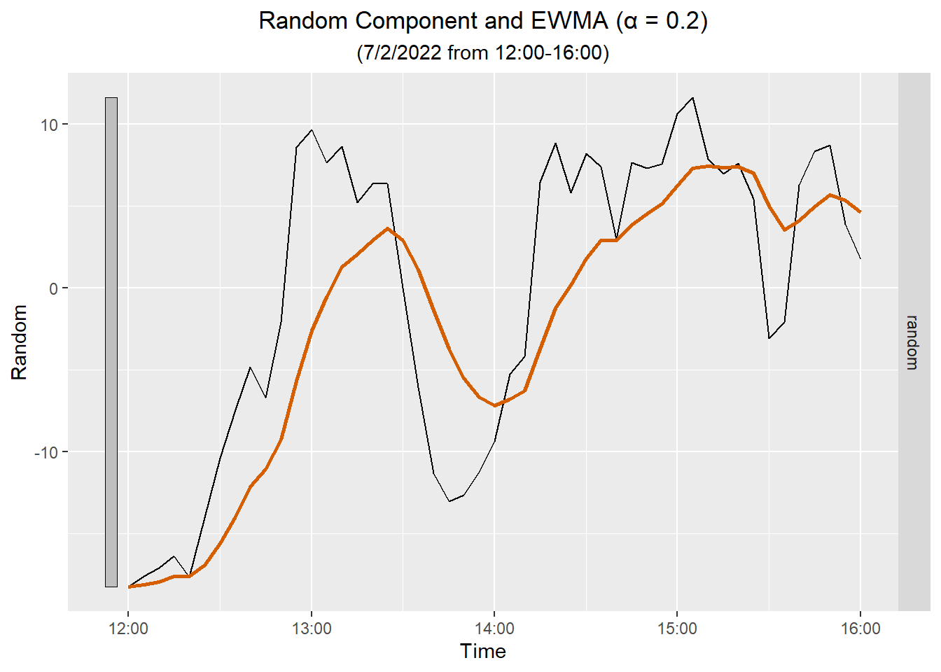
Table 4: Illustration of the computation of the EWMA

Date-Time	Random $$ \hat z_t $$	Computation of $$ a_t $$	$$a_t$$
7/2/2022 12:00	-18.258	-18.258 =	-18.258
7/2/2022 12:05	-17.597	0.2 * (-17.597) + (1 - 0.2) * (-18.258) =	-18.126
7/2/2022 12:10	-17.095	0.2 * (-17.095) + (1 - 0.2) * (-18.126) =	-17.919
7/2/2022 12:15	-16.342	0.2 * (-16.342) + (1 - 0.2) * (-17.919) =	-17.604
7/2/2022 12:20	-17.627	0.2 * (-17.627) + (1 - 0.2) * (-17.604) =	-17.608
7/2/2022 12:25	-14.03	0.2 * (-14.03) + (1 - 0.2) * (-17.608) =	-16.893

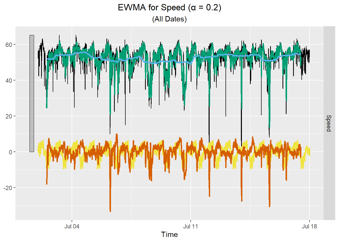
Here is a plot showing the EWMA for the random component for all the data.

Figure 10: EWMA superimposed on the random component of the traffic data time series

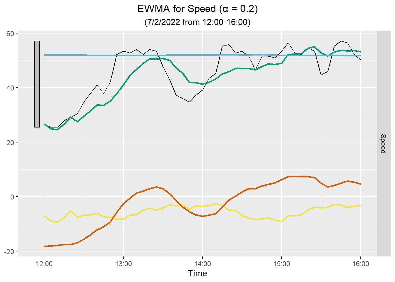
Here is a plot of the EWMA against the random component for four hours:

Figure 11: EWMA superimposed on the random component of the traffic data for a four-hour period

EWMA with \(\alpha = 0.75\)

EWMA

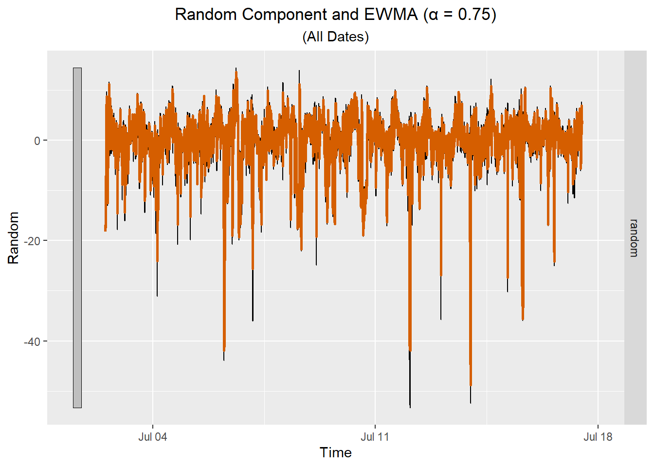
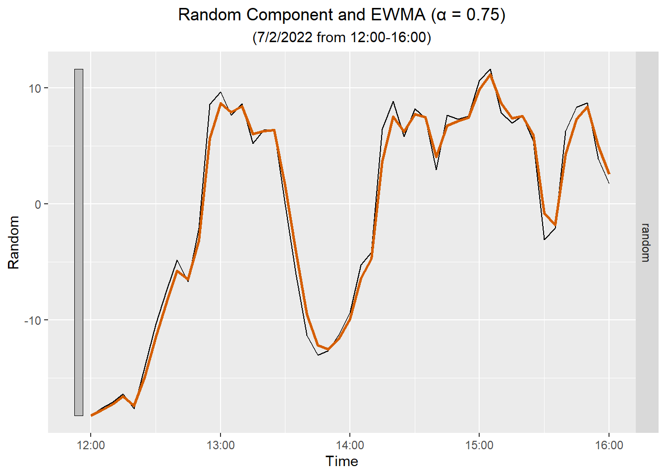
Table 5: Illustration of the computation of the EWMA

Date-Time	Random $$ \hat z_t $$	Computation of $$ a_t $$	$$a_t$$
7/2/2022 12:00	-18.258	-18.258 =	-18.258
7/2/2022 12:05	-17.597	0.75 * (-17.597) + (1 - 0.75) * (-18.258) =	-17.762
7/2/2022 12:10	-17.095	0.75 * (-17.095) + (1 - 0.75) * (-17.762) =	-17.261
7/2/2022 12:15	-16.342	0.75 * (-16.342) + (1 - 0.75) * (-17.261) =	-16.572
7/2/2022 12:20	-17.627	0.75 * (-17.627) + (1 - 0.75) * (-16.572) =	-17.363
7/2/2022 12:25	-14.03	0.75 * (-14.03) + (1 - 0.75) * (-17.363) =	-14.864

Here is a plot showing the EWMA for the random component for all the data.

Figure 12: EWMA superimposed on the random component of the traffic data time series

Here is a plot of the EWMA against the random component for four hours:

Figure 13: EWMA superimposed on the random component of the traffic data for a four-hour period

Once we have obtained the EWMA for the random component, we can add to it the trend and seasonality to get the EWMA for the original speed data. The raw data are plotted in black, the trend in blue, the seasonal component in yellow, and the EWMA is plotted in orange. The green curve is the sum of EWMA, the seasonal component, and the trend.

Figure 14: Components of the EWMA superimposed on the random component of the New York traffic data

Here is the plot for four hours of data:

Figure 15: Components of the EWMA superimposed on the random component of the New York traffic data, four hours only

Class Activity: EWMA in R (10 min)

We will compute the EWMA for the random component of the New York highway speed data in R. We have already decomposed the model, so we have isolated the estimated values for the random component. This is a portion of the tsibble ny_speeds_decompose:

Table 6: A portion of the tsibble containing the EWMA for the random component of the traffic data

.model	index	speed	trend	seasonal	random	season_adjust
feasts::classical_decomposition(speed ~ season(288), type = "add")	2022-07-02	52.19	NA	2.557	NA	49.633
feasts::classical_decomposition(speed ~ season(288), type = "add")	2022-07-02 00:05:00	53.43	NA	2.884	NA	50.546
feasts::classical_decomposition(speed ~ season(288), type = "add")	2022-07-02 00:10:00	55.92	NA	2.463	NA	53.457
⋮	⋮	⋮	⋮	⋮	⋮	⋮
feasts::classical_decomposition(speed ~ season(288), type = "add")	2022-07-02 11:55:00	30.44	NA	-4.195	NA	34.635
feasts::classical_decomposition(speed ~ season(288), type = "add")	2022-07-02 12:00:00	26.71	51.969	-7.002	-18.258	33.712
feasts::classical_decomposition(speed ~ season(288), type = "add")	2022-07-02 12:05:00	25.47	51.973	-8.906	-17.597	34.376
feasts::classical_decomposition(speed ~ season(288), type = "add")	2022-07-02 12:10:00	25.47	51.969	-9.405	-17.095	34.875
⋮	⋮	⋮	⋮	⋮	⋮	⋮
feasts::classical_decomposition(speed ~ season(288), type = "add")	2022-07-17 11:45:00	53.43	54.612	-4.153	2.971	57.583
feasts::classical_decomposition(speed ~ season(288), type = "add")	2022-07-17 11:50:00	54.05	54.616	-4.485	3.918	58.535
feasts::classical_decomposition(speed ~ season(288), type = "add")	2022-07-17 11:55:00	53.43	54.626	-4.195	2.999	57.625
feasts::classical_decomposition(speed ~ season(288), type = "add")	2022-07-17 12:00:00	50.33	NA	-7.002	NA	57.332
⋮	⋮	⋮	⋮	⋮	⋮	⋮
feasts::classical_decomposition(speed ~ season(288), type = "add")	2022-07-17 23:45:00	55.3	NA	-1.237	NA	56.537
feasts::classical_decomposition(speed ~ season(288), type = "add")	2022-07-17 23:50:00	55.92	NA	-1.905	NA	57.825
feasts::classical_decomposition(speed ~ season(288), type = "add")	2022-07-17 23:55:00	57.16	NA	1.528	NA	55.632

Warning

When applying EWMA to the random component of the time series, delete the variable .model and all NA values from the data frame. If you neglect this step, there will be errors in the code below.

We drop the variable .model and omit all NA values. (Remember the first half-day and the last half-day in the time series do not yield estimates for the random component.)

ny_speeds_random <- ny_speeds_decompose |>
  na.omit() |>                                # Omit all NA values
  select(-.model)                             # Eliminate the variable .model

The following code can be used to execute the EWMA algorithm on the random component using \(\alpha = 0.2\).

ny_speeds_model1 <- ny_speeds_random |>
  model(Additive = ETS(random ~
                         trend("A", alpha = 0.2, beta = 0) +
                         error("A") + season("N"),
                       opt_crit = "amse", nmse = 1))
report(ny_speeds_model1)

Series: random 
Model: ETS(A,A,N) 
  Smoothing parameters:
    alpha = 0.2 
    beta  = 0 

  Initial states:
      l[0]        b[0]
 -13.52924 0.003643793

  sigma^2:  22.2348

     AIC     AICc      BIC 
49563.94 49563.94 49583.05 

Now, we calculate the value of SS1PE.

sum(components(ny_speeds_model1)$remainder^2, na.rm = TRUE)

[1] 95965.59

Check Your Understanding

• Modify the code analyzing the New York traffic speed data by deleting the argument alpha = 0.2.
  • What value of \(\alpha\) is obtained?
  • What is the value of the SS1PE for this value of \(\alpha\)?
• Choose values of \(\alpha\) slightly less than and slightly greater than 0.6722.
  • Can you find a value of \(\alpha\) that gives you a smaller SS1PE than 77661.59?

Homework Preview (5 min)

• Review upcoming homework assignment
• Clarify questions

Download Homework

homework_3_2.qmd

Matching Activity

Solutions to matching activity:

1. D
2. E
3. B
4. C
5. A

Class Activity: Practice Applying the EWMA

Table 7: Calculation of \(a_t\) and \(e_t\) for a sample time series: Solution for Table 1

$$t$$	$$x_t$$	$$a_t$$	$$e_t$$
$$ 1 $$	$$ 4.4 $$	$$4.4$$
$$ 2 $$	$$ 4.2 $$	$$ 0.2 \cdot 4.2 + (1 - 0.2 ) \cdot 4.4 = 4.36 $$	$$ 4.2 - 4.4 = -0.2 $$
$$ 3 $$	$$ 4.2 $$	$$ 0.2 \cdot 4.2 + (1 - 0.2 ) \cdot 4.36 = 4.328 $$	$$ 4.2 - 4.36 = -0.16 $$
$$ 4 $$	$$ 4 $$	$$ 0.2 \cdot 4 + (1 - 0.2 ) \cdot 4.328 = 4.262 $$	$$ 4 - 4.328 = -0.328 $$
$$ 5 $$	$$ 4.4 $$	$$ 0.2 \cdot 4.4 + (1 - 0.2 ) \cdot 4.262 = 4.29 $$	$$ 4.4 - 4.262 = 0.138 $$
$$ 6 $$	$$ 4.7 $$	$$ 0.2 \cdot 4.7 + (1 - 0.2 ) \cdot 4.29 = 4.372 $$	$$ 4.7 - 4.29 = 0.41 $$
$$ 7 $$	$$ 4.9 $$	$$ 0.2 \cdot 4.9 + (1 - 0.2 ) \cdot 4.372 = 4.478 $$	$$ 4.9 - 4.372 = 0.528 $$
$$ 8 $$	$$ 5.3 $$	$$ 0.2 \cdot 5.3 + (1 - 0.2 ) \cdot 4.478 = 4.642 $$	$$ 5.3 - 4.478 = 0.822 $$
$$ 9 $$	$$ 5.4 $$	$$ 0.2 \cdot 5.4 + (1 - 0.2 ) \cdot 4.642 = 4.794 $$	$$ 5.4 - 4.642 = 0.758 $$
$$ 10 $$	$$ 5.5 $$	$$ 0.2 \cdot 5.5 + (1 - 0.2 ) \cdot 4.794 = 4.935 $$	$$ 5.5 - 4.794 = 0.706 $$

The value of SS1PE is \[ \sum\limits_{t=2}^n e_t^2 = (-0.2)^2 + (-0.16)^2 + \cdots + (0.758)^2 + (0.706)^2 = 2.389 \]