Holt-Winters Method (Additive Models) - Part 2

Chapter 3: Lesson 4

Learning Outcomes

Implement the Holt-Winter method to forecast time series

• Compute the Holt-Winters estimate by hand
• Use HoltWinters() to forecast additive model time series
• Plot the Holt-Winters decomposition of a time series (see Fig 3.10)
• Plot the Holt-Winters fitted values versus the original time series (see Fig 3.11)
• Superimpose plots of the Holt-Winters predictions with the time series realizations (see Fig 3.13)

Preparation

• Review Section 3.4.2 (Page 59 - top of page 60 only)

Learning Journal Exchange (10 min)

• Review another student’s journal

• What would you add to your learning journal after reading another student’s?

• What would you recommend the other student add to their learning journal?

• Sign the Learning Journal review sheet for your peer

Packages

# Extra packages this lesson
pacman::p_load(nanoparquet) # parquet files load faster
# rio will use this automatically if it's installed

pacman::p_load(
  tidyverse,  # ggplot, mutate(), cleaning...
  tsibble,    # as_tsibble()
  fable,      # model(...), forecast(), tidy(), glance()...
  feasts,     # ACF(), PACF()
  ggtime,     # autoplot() for tsibbles
  patchwork,  # + and / for ggplots
  rio         # import()
)

Small Group Activity: Holt-Winters Model for Residential Natural Gas Consumption (35 min)

The United States Energy Information Administration (EIA) publishes data on the total residential natural gas consumption in the country. This government agency publishes monthly data beginning in January 1973. For the purpose of this example, we will only consider quarterly values beginning in 2017. The data are given in MMcf (thousand-thousand cubic feet, or millions of cubic feet). We convert the data to billions of cubic feet (Bcf) and round to the nearest integer to make the numbers a little more manageable.

nat_gas <- rio::import("https://byuistats.github.io/timeseries/data/natural_gas_res.csv") |>
  mutate(date = my(month)) |>
  filter(date >= my("Jan 2017")) |>
  mutate(quarter = yearquarter(date)) |>
  group_by(quarter) |> 
  summarize(
    gas_use_mmcf = sum(residential_nat_gas_consumption),
    n = n()
  ) |>
  filter(n == 3) |>  # Eliminate partial quarter(s)
  dplyr::select(-n) |>
  mutate(gas_billion_cf = round(gas_use_mmcf / 10^3))

quarter	gas_use_mmcf	gas_billion_cf
2017 Q1	1990316	1990
2017 Q2	602515	603
2017 Q3	325786	326
2017 Q4	1494706	1495
2018 Q1	2330552	2331
2018 Q2	729111	729
⋮	⋮	⋮
2022 Q2	709645	710
2022 Q3	327101	327
2022 Q4	1590005	1590
2023 Q1	2114999	2115
2023 Q2	663003	663
2023 Q3	328735	329

The quarters are defined as:

• Quarter 1: Jan, Feb, Mar
• Quarter 2: Apr, May, Jun
• Quarter 3: Jul, Aug, Sep
• Quarter 4: Oct, Nov, Dec

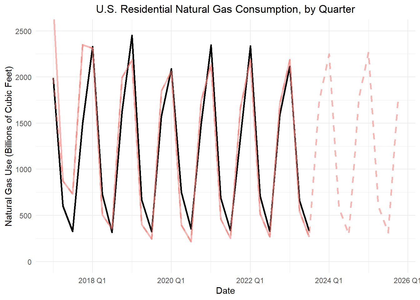
The weather is colder in the first and fourth quarters, so the demand for natural gas will be higher then. As illustrated in Figure 1, the difference in the consumption in the lowest and highest quarters of a year tends to be about 2000 Bcf.

Figure 1: Quarterly U.S. natural gas consumption (Bcf)

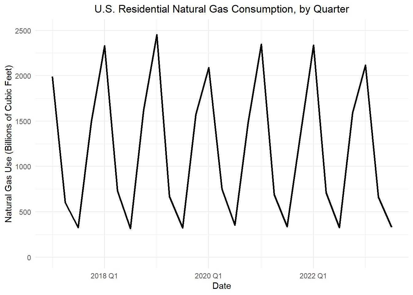
We will use this information to create an initial estimate of the seasonality of the time series. We will assume that in Quarters 1 and 4, natural gas use is 1000 Bcf above the level of the time series and in Quarters 2 and 3, it is 1000 Bcf below the level of the time series. This is not accurate, but it gives us a reasonable starting point.

The portion of the time series we are using begins in the first quarter of 2017. So we will choose the initial values of \(s_t\) as: \[ s_{Q1} = 1000, ~~~ s_{Q2} = -1000, ~~~ s_{Q3} = -1000, ~~~ s_{Q4} = 1000 \]

With \(p=4\) quarters in a year, we implement initial seasonality estimates in the Holt-Winters model as \[ s_{1-p} = s_{(-3)} = 1000, ~~~ s_{2-p} = s_{(-2)} = -1000, ~~~ s_{3-p} = s_{(-1)} = -1000, ~~~ s_{4-p} = s_{0} = 1000 \]

Tables-Handout-Excel

for parameter values reference the “check your understanding” section below this table

Table 1: Holt-Winters filter for the quarterly natural gas consumption in the U.S. in billions of cubic feet

$$Quarter$$	$$t$$	$$x_t$$	$$a_t$$	$$b_t$$	$$s_t$$	$$\hat x_t$$
2016 Q1	-3	—	—	—	1000	—
2016 Q2	-2	—	—	—	-1000	—
2016 Q3	-1	—	—	—	-1000	—
2016 Q4	0	—	—	—	1000	—
2017 Q1	1	1990
2017 Q2	2	603
2017 Q3	3	326
2017 Q4	4	1495
2018 Q1	5	2331	1508	-58	805	2313
2018 Q2	6	729	1519	-44	-1012	507
2018 Q3	7	318	1464	-46	-1110	354
2018 Q4	8	1620	1301	-69	693	1994
2019 Q1	9	2451	1315	-52	871	2186
2019 Q2	10	670	1347	-35	-945	402
2019 Q3	11	323	1336	-30	-1091	245
2019 Q4	12	1573	1221	-47	625	1846
2020 Q1	13	2089	1183	-45	878	2061
2020 Q2	14	751	1250	-23	-856	394
2020 Q3	15	354	1271	-14	-1056	215
2020 Q4	16	1481	1177	-30	561	1738
2021 Q1	17	2345	1211	-17	929	2140
2021 Q2	18	690	1264	-3	-800	464
2021 Q3	19	338	1288	2	-1035	253
2021 Q4	20	1344	1189	-18	480	1669
2022 Q1	21	2337	1218	-9	967	2185
2022 Q2	22	710	1269	3	-752	517
2022 Q3	23	327	1290	7	-1021	269
2022 Q4	24	1590	1260	0	450
2023 Q1	25	2115	1238	-4	949
2023 Q2	26	663	1270	3	-723
2023 Q3	27	329	1288	6	-1021
2023 Q4	28	—	—	—
2024 Q1	29	—	—	—
2024 Q2	30	—	—	—
2024 Q3	31	—	—	—
2024 Q4	32	—	—	—
2025 Q1	33	—	—	—
2025 Q2	34	—	—	—
2025 Q3	35	—	—	—
2025 Q4	36	—	—	—

NoteHolt-Winters Update Equations (Additive Model)

Recall the three Holt-Winters update equations for an additive model are:

\[\begin{align*} a_t &= \alpha \left( x_t - s_{t-p} \right) + (1-\alpha) \left( a_{t-1} + b_{t-1} \right) && \text{Level} \\ b_t &= \beta \left( a_t - a_{t-1} \right) + (1-\beta) b_{t-1} && \text{Slope} \\ s_t &= \gamma \left( x_t - a_t \right) + (1-\gamma) s_{t-p} && \text{Seasonal} \end{align*}\]

where \(\{x_t\}\) is a time series from \(t=1\) to \(t=n\) that has seasonality with a period of \(p\) time units; at time \(t\), \(a_t\) is the estimated level of the time series, \(b_t\) is the estimated slope, and \(s_t\) is the estimated seasonal component; and \(\alpha\), \(\beta\), and \(\gamma\) are parameters (all between 0 and 1).

The forecasting equation is: \[ \hat x_{n+k|n} = a_n + k b_n + s_{n+k-p} \]

The details of these computations are given in Chapter 3 Lesson 3.

Note

For \(k = 0\) : \[ \hat x_{n} = a_n + 0 b_n + s_{n+-p} \]

\[ = a_n + s_{n+k-p} \]

TipCheck Your Understanding

Apply Holt-Winters filtering to these data. Use \(\alpha = \beta = \gamma = 0.2\).

• Find \(a_1\)
• Find \(b_1\)
• Compute the missing values of \(a_t\), \(b_t\), and \(s_t\) for all quarters from Q1 of 2017 to the end of the data set.
• Find \(\hat x_t\) for all rows where \(t \ge 1\). Note that the expression to compute \(\hat x_t\) is different for the rows with data versus the rows where forecasting is required.
• Superimpose a sketch of your Holt-Winters filter and the associated forecast on Figure 1.

Small Group Activity: Application of Holt-Winters in R using the Baltimore Crime Data (20 min)

Background

The City of Baltimore publishes crime data, which can be accessed through a query. This dataset is sourced from the City of Baltimore Open Data. You can explore the data on data.world.

Use the following code to import the data:

crime_df <- rio::import("https://byuistats.github.io/timeseries/data/baltimore_crime.parquet")

The data set consists of 285807 rows and 12 columns. There are a few key variables:

• Date and Time: Records the date and time of each incident.
• Location: Detailed coordinates of each incident.
• Crime Type: Description of the type of crime.

When exploring a new time series, it is crucial to carefully examine the data. Here are a few rows of the original data set. Note that the data are not sorted in time order.

CrimeDate	CrimeTime	CrimeCode	Location	Description	Inside.Outside	Weapon	Post	District	Neighborhood	Location.1	Total.Incidents
11/12/2016	02:35:00	3B	300 SAINT PAUL PL	ROBBERY - STREET	O	NA	111	CENTRAL	Downtown	(39.2924100000, -76.6140800000)	1
11/12/2016	02:56:00	3CF	800 S BROADWAY	ROBBERY - COMMERCIAL	I	FIREARM	213	SOUTHEASTERN	Fells Point	(39.2824200000, -76.5928800000)	1
11/12/2016	03:00:00	6D	1500 PENTWOOD RD	LARCENY FROM AUTO	O	NA	413	NORTHEASTERN	Stonewood-Pentwood-Winston	(39.3480500000, -76.5883400000)	1
11/12/2016	03:00:00	6D	6600 MILTON LN	LARCENY FROM AUTO	O	NA	424	NORTHEASTERN	Westfield	(39.3626300000, -76.5516100000)	1
11/12/2016	03:00:00	6E	300 W BALTIMORE ST	LARCENY	O	NA	111	CENTRAL	Downtown	(39.2893800000, -76.6197100000)	1
11/12/2016	03:00:00	4E	6900 MCCLEAN BLVD	COMMON ASSAULT	I	HANDS	423	NORTHEASTERN	Hamilton Hills	(39.3707000000, -76.5670900000)	1
⋮	⋮	⋮	⋮	⋮	⋮	⋮	⋮	⋮	⋮	⋮	⋮
01/01/2011	23:00:00	7A	2500 ARUNAH AV	AUTO THEFT	O	NA	721	WESTERN	Evergreen Lawn	(39.2954200000, -76.6592800000)	1
01/01/2011	23:25:00	4E	100 N MONROE ST	COMMON ASSAULT	I	HANDS	714	WESTERN	Penrose/Fayette Street Outreach	(39.2899900000, -76.6470700000)	1
01/01/2011	23:38:00	4D	800 N FREMONT AV	AGG. ASSAULT	I	HANDS	123	WESTERN	Upton	(39.2981200000, -76.6339100000)	1

TipCheck Your Understanding

• Using the command crime_df |> summary(), we learn that the Total.Incidents always equals 1. What does each row in the data frame represent?

We now summarize the data into a daily tsibble.

# Data Summary and Aggregation
# Group by dates column and summarize from Total.Incidents column
daily_summary_df <- crime_df |>
  rename(dates = CrimeDate) |>
  group_by(dates) |>
  summarise(incidents = sum(Total.Incidents))

# Data Transformation and Formatting
# Select relevant columns, format dates, and arrange the data
crime_data <- daily_summary_df |>
  mutate(dates = mdy(dates)) |>
  mutate(
    month = month(dates),
    day = day(dates),
    year = year(dates)
  ) |>
  arrange(dates) |>
  dplyr::select(dates, month, day, year, incidents)
  
# Convert formatted data to a tsibble with dates as the index
crime_tsibble <- as_tsibble(crime_data, index = dates) 

Here are a few rows of the data after summing the crime incidents each day.

dates	month	day	year	incidents
2011-01-01	1	1	2011	185
2011-01-02	1	2	2011	102
2011-01-03	1	3	2011	106
2011-01-04	1	4	2011	113
2011-01-05	1	5	2011	131
2011-01-06	1	6	2011	107
⋮	⋮	⋮	⋮	⋮
2016-11-10	11	10	2016	109
2016-11-11	11	11	2016	115
2016-11-12	11	12	2016	69

Here is a time plot of the number of crimes reported in Baltimore daily.

# Time series plot of total incidents over time
crime_plot <- autoplot(crime_tsibble, .vars = incidents) +
  labs(
    x = "Time",
    y = "Total Crime Incidents",
    title = "Total Crime Incidents Over Time"
  ) +
  theme(plot.title = element_text(hjust = 0.5))

# Display the plot
crime_plot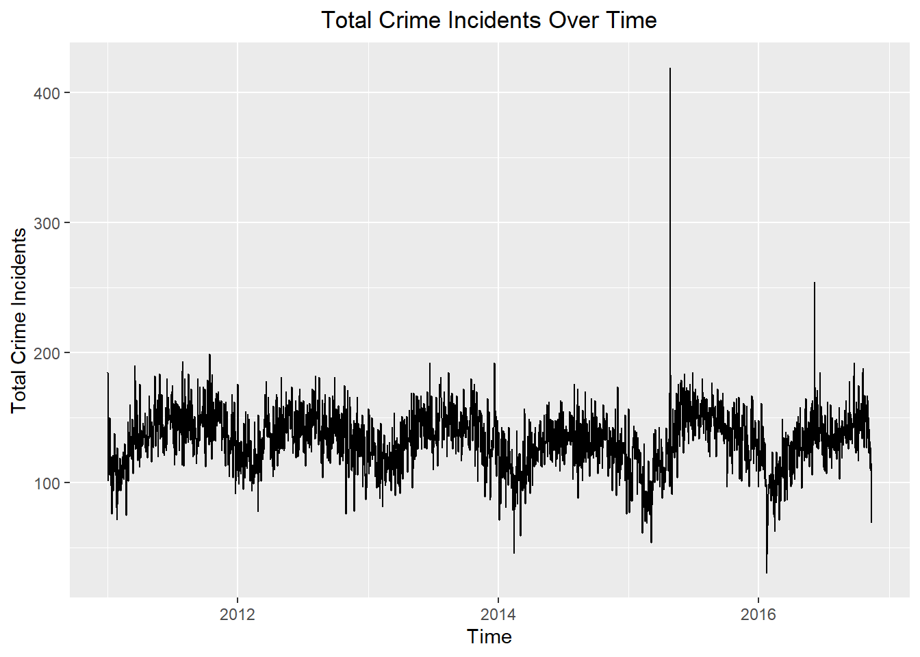

TipCheck Your Understanding

• What do you notice about this time plot?
  • Describe the trend
  • Is there evidence of seasonality?
  • Is the additive or multiplicative model appropriate?
  • Which date has the highest number of recorded crimes? Can you determine a reason for this spike?

The following table summarizes the number of days in each month for which crime data were reported.

crime_data |>
  mutate(month_char = format(as.Date(dates), '%b') ) |>
  group_by(month, month_char, year) |>
  summarise(n = n(), .groups = "keep") |>
  group_by() |>
  arrange(year, month) |>
  dplyr::select(-month) |>
  rename(Year = year) |>
  pivot_wider(names_from = month_char, values_from = n) |>
  display_table()

Year	Jan	Feb	Mar	Apr	May	Jun	Jul	Aug	Sep	Oct	Nov	Dec
2011	31	28	31	30	31	30	31	31	30	31	30	31
2012	31	29	31	30	31	30	31	31	30	31	30	31
2013	31	28	31	30	31	30	31	31	30	31	30	31
2014	31	28	31	30	31	30	31	31	30	31	30	31
2015	31	28	31	30	31	30	31	31	30	31	30	31
2016	31	29	31	30	31	30	31	31	30	31	12	NA

TipCheck Your Understanding

• What do you observe about the data?
• What are some problems that could arise from incomplete data?
• How do you recommend we address the missing data?

Monthly Summary

We could analyze the data at the daily level, but for simplicity we will model the monthly totals.

crime_monthly_ts <- crime_tsibble |>
  as_tibble() |>
  mutate(months = yearmonth(dates)) |>
  group_by(months) |>
  summarize(value = sum(incidents)) |>
  as_tsibble(index = months) 

# Plot mean annual total incidents using autoplot
autoplot(crime_monthly_ts, .vars = value) +
  labs(
    x = "Year",
    y = "Total Monthly Crime Incidents",
  ) +
  theme(plot.title = element_text(hjust = 0.5))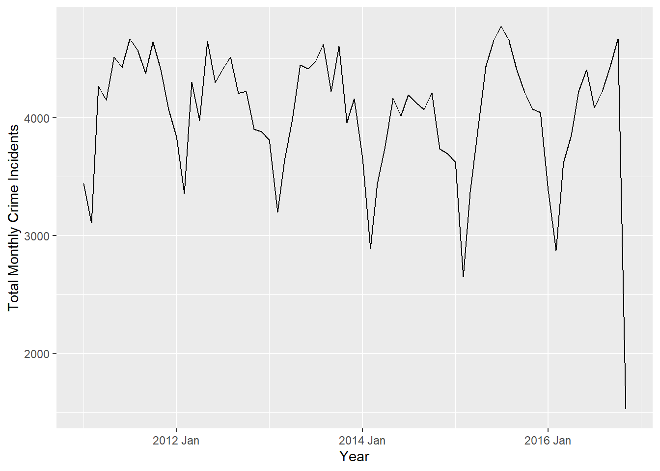

There is incomplete data for 2016, as data were not provided after 11/12/2016. We will omit any data after October 2016.

crime_monthly_ts1 <- crime_monthly_ts |>
  filter(months < yearmonth(mdy("11/1/2016")))

We apply Holt-Winters filtering on the monthly Baltimore crimes data with an additive model:

crime_hw <- crime_monthly_ts1 |>
  tsibble::fill_gaps() |>
  model(Additive = ETS(value ~
        trend("A") +
        error("A") +
        season("A"),
        opt_crit = "amse", nmse = 1))
report(crime_hw)

Series: value 
Model: ETS(A,A,A) 
  Smoothing parameters:
    alpha = 0.4102911 
    beta  = 0.0001719 
    gamma = 0.001008159 

  Initial states:
     l[0]      b[0]      s[0]     s[-1]    s[-2]    s[-3]    s[-4]    s[-5]
 4318.875 -4.475258 -83.12823 -38.36167 374.3369 217.8943 416.0997 428.0887
    s[-6]    s[-7]     s[-8]     s[-9]    s[-10]    s[-11]
 301.8743 366.7473 -141.8365 -334.7158 -1039.907 -467.0918

  sigma^2:  45518.72

     AIC     AICc      BIC 
1064.040 1075.810 1102.265 

We can compute some values to assess the fit of the model:

# SS of random terms
sum(components(crime_hw)$remainder^2, na.rm = T)

# RMSE
forecast::accuracy(crime_hw)$RMSE

# Standard devation of number of incidents each month
sd(crime_monthly_ts1$value)

• The sum of the square of the random terms is: 2.4580111^{6}.
• The root mean square error (RMSE) is: 187.388486.
• The standard deviation of the number of incidents each month is 22.9761197.

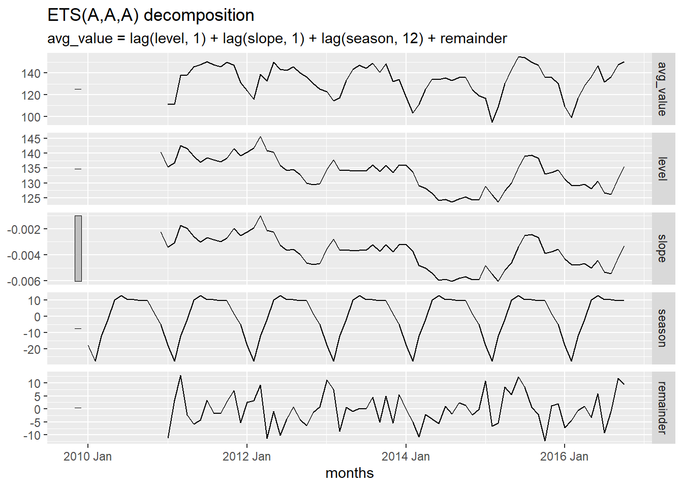
Figure 2 illustrates the Holt-Winters decomposition of the Baltimore crime data.

autoplot(components(crime_hw))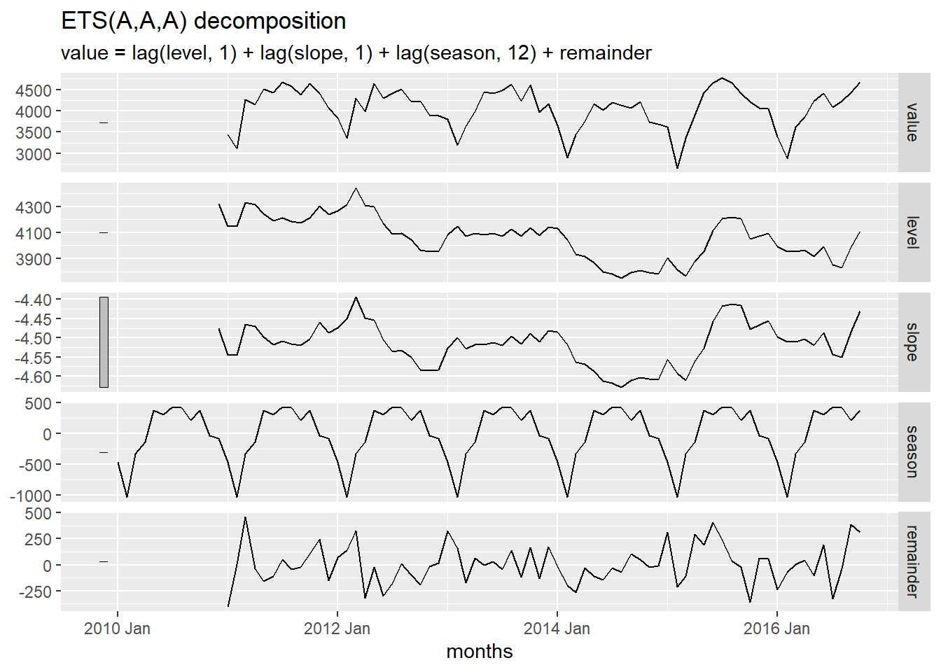

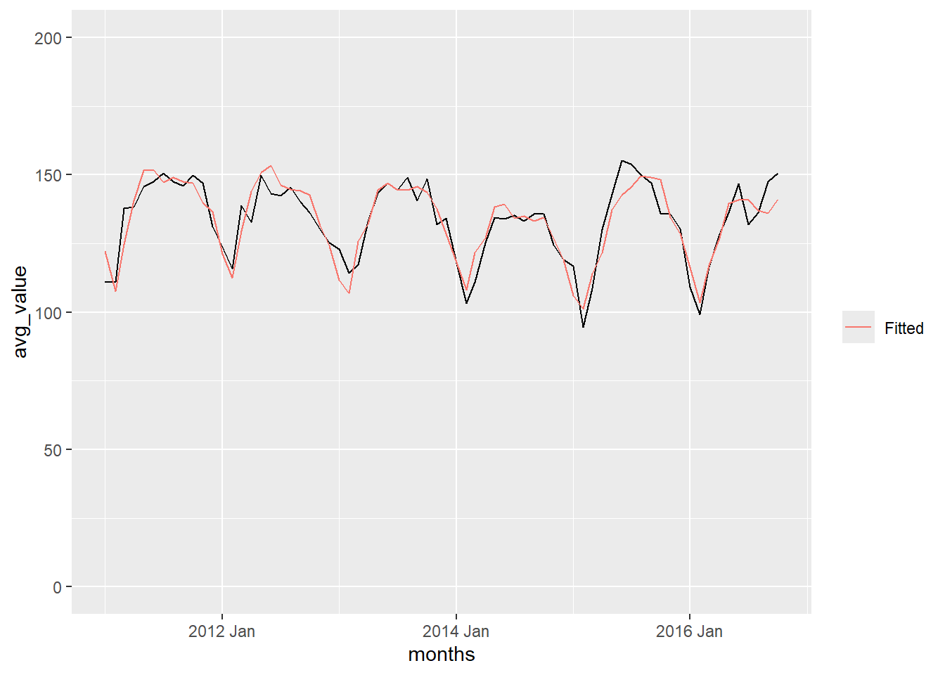
Figure 2: Monthly Total Number of Crime Reported in Baltimore

In Figure 3, we can observe the relationship between the Holt-Winters filter and the time series of the number of crimes each month.

augment(crime_hw) |>
  ggplot(aes(x = months, y = value)) +
    coord_cartesian(ylim = c(0,5500)) +
    geom_line() +
    geom_line(aes(y = .fitted, color = "Fitted")) +
    labs(color = "")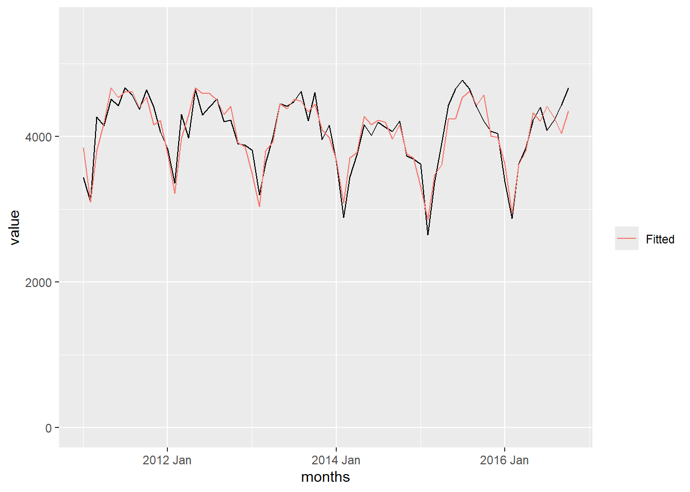

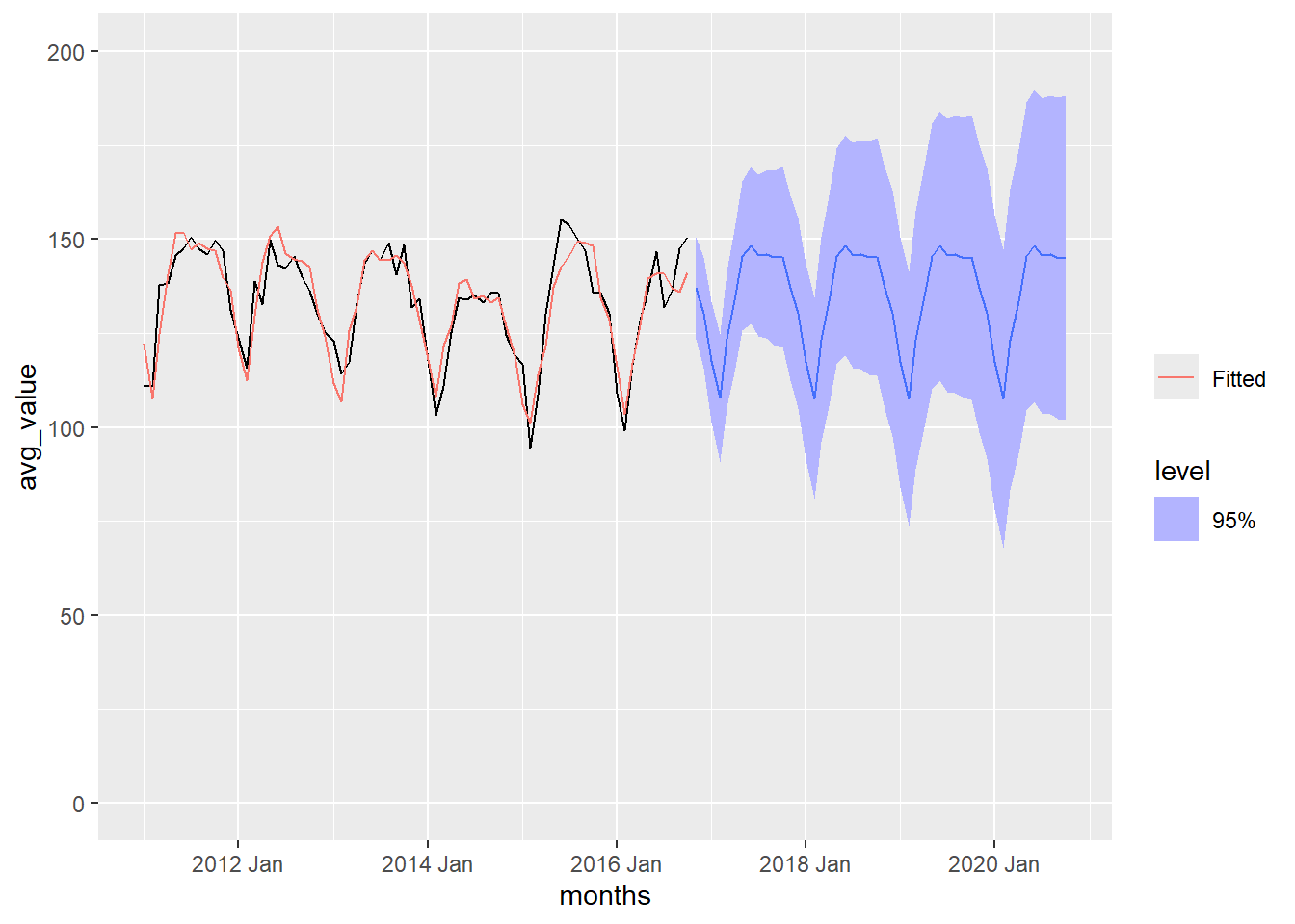
Figure 3: Superimposed plots of the number of crimes each month and the Holt-Winters filter

Figure 4 contains the information from Figure 3, with the addition of an additional four years of forecasted values. The light blue bands give the 95% prediction bands for the forecast.

crime_forecast <- crime_hw |>
  forecast(h = "4 years") 
crime_forecast |>
  autoplot(crime_monthly_ts1, level = 95) +
  coord_cartesian(ylim = c(0,5500)) +
  geom_line(aes(y = .fitted, color = "Fitted"),
    data = augment(crime_hw)) +
  scale_color_discrete(name = "")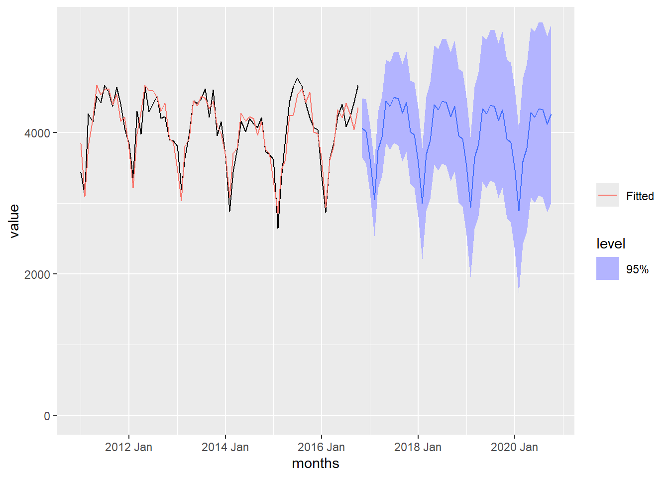

Figure 4: Superimposed plots of the number of crimes each month and the Holt-Winters filter, with four additional years forecasted

Rethinking Baltimore

The monthly crime data shows a distinct pattern arcing through the annual cycle. Consider the data for 2011.

Table 2: Total count of crimes reported in Baltimore in 2011 by month

Jan	Feb	Mar	Apr	May	Jun	Jul	Aug	Sep	Oct	Nov	Dec
3440	3108	4269	4149	4516	4427	4669	4574	4377	4644	4411	4067

TipCheck Your Understanding

• Starting with January, determine whether the number of crimes goes up or down as you move from one month to the next.
• What might explain this pattern?
• Use the function days_in_month() to adjust the time series and re-run the analysis. What do you notice?

Homework Preview (5 min)

• Review upcoming homework assignment
• Clarify questions

NoteDownload Homework

homework_3_4.qmd

Natural Gas Holt-Winters Filter

Tables-Handout-Excel-key

Quarterly U.S. natural gas consumption (Bcf)

Holt-Winters filter for the quarterly natural gas consumption in the U.S. in billions of cubic feet

$$Quarter$$	$$t$$	$$x_t$$	$$a_t$$	$$b_t$$	$$s_t$$	$$\hat x_t$$
2016 Q1	-3	—	—	—	1000	—
2016 Q2	-2	—	—	—	-1000	—
2016 Q3	-1	—	—	—	-1000	—
2016 Q4	0	—	—	—	1000	—
2017 Q1	1	1990	1990	36	800	1990
2017 Q2	2	603	1941	19	-1068	873
2017 Q3	3	326	1833	-6	-1101	732
2017 Q4	4	1495	1561	-59	787	2348
2018 Q1	5	2331	1508	-58	805	2313
2018 Q2	6	729	1519	-44	-1012	507
2018 Q3	7	318	1464	-46	-1110	354
2018 Q4	8	1620	1301	-69	693	1994
2019 Q1	9	2451	1315	-52	871	2186
2019 Q2	10	670	1347	-35	-945	402
2019 Q3	11	323	1336	-30	-1091	245
2019 Q4	12	1573	1221	-47	625	1846
2020 Q1	13	2089	1183	-45	878	2061
2020 Q2	14	751	1250	-23	-856	394
2020 Q3	15	354	1271	-14	-1056	215
2020 Q4	16	1481	1177	-30	561	1738
2021 Q1	17	2345	1211	-17	929	2140
2021 Q2	18	690	1264	-3	-800	464
2021 Q3	19	338	1288	2	-1035	253
2021 Q4	20	1344	1189	-18	480	1669
2022 Q1	21	2337	1218	-9	967	2185
2022 Q2	22	710	1269	3	-752	517
2022 Q3	23	327	1290	7	-1021	269
2022 Q4	24	1590	1260	0	450	1710
2023 Q1	25	2115	1238	-4	949	2187
2023 Q2	26	663	1270	3	-723	547
2023 Q3	27	329	1288	6	-1021	267
2023 Q4	28	—	—	—	450	1744
2024 Q1	29	—	—	—	949	2249
2024 Q2	30	—	—	—	-723	583
2024 Q3	31	—	—	—	-1021	291
2024 Q4	32	—	—	—	450	1768
2025 Q1	33	—	—	—	949	2273
2025 Q2	34	—	—	—	-723	607
2025 Q3	35	—	—	—	-1021	315
2025 Q4	36	—	—	—	450	1792

Balitmore Crime Spike

# Dates with high criminal activity
crime_data |> arrange(desc(incidents)) |> head()

# A tibble: 6 × 5
  dates      month   day  year incidents
  <date>     <dbl> <int> <dbl>     <dbl>
1 2015-04-27     4    27  2015       419
2 2016-06-05     6     5  2016       254
3 2011-10-14    10    14  2011       199
4 2011-07-30     7    30  2011       193
5 2013-06-22     6    22  2013       192
6 2013-12-20    12    20  2013       192

On April 27, 2015, 419 crimes were recorded. These are associated with protests over arrest of Freddie Gray.

Balitmore (Mean Crimes Per Day)

crime_monthly_ts2 <- crime_monthly_ts1 |> 
  mutate(avg_value = value / days_in_month(ym(months))) |>
  dplyr::select(-value)

crime_hw2 <- crime_monthly_ts2 |>
  tsibble::fill_gaps() |>
  model(Additive = ETS(avg_value ~
        trend("A") +
        error("A") +
        season("A"),
        opt_crit = "amse", nmse = 1))
report(crime_hw)

Series: value 
Model: ETS(A,A,A) 
  Smoothing parameters:
    alpha = 0.4102911 
    beta  = 0.0001719 
    gamma = 0.001008159 

  Initial states:
     l[0]      b[0]      s[0]     s[-1]    s[-2]    s[-3]    s[-4]    s[-5]
 4318.875 -4.475258 -83.12823 -38.36167 374.3369 217.8943 416.0997 428.0887
    s[-6]    s[-7]     s[-8]     s[-9]    s[-10]    s[-11]
 301.8743 366.7473 -141.8365 -334.7158 -1039.907 -467.0918

  sigma^2:  45518.72

     AIC     AICc      BIC 
1064.040 1075.810 1102.265 

autoplot(components(crime_hw2))

Figure 5: Monthly Total Number of Crime Reported in Baltimore

augment(crime_hw2) |>
  ggplot(aes(x = months, y = avg_value)) +
    coord_cartesian(ylim = c(0,200)) +
    geom_line() +
    geom_line(aes(y = .fitted, color = "Fitted")) +
    labs(color = "")

Figure 6: Superimposed plots of the number of crimes each month and the Holt-Winters filter

Figure 4 contains the information from Figure 3, with the addition of an additional four years of forecasted values. The light blue bands give the 95% prediction bands for the forecast.

crime_forecast <- crime_hw2 |>
  forecast(h = "4 years") 
crime_forecast |>
  autoplot(crime_monthly_ts2, level = 95) +
  coord_cartesian(ylim = c(0,200)) +
  geom_line(aes(y = .fitted, color = "Fitted"),
    data = augment(crime_hw2)) +
  scale_color_discrete(name = "")

Figure 7: Superimposed plots of the number of crimes each month and the Holt-Winters filter, with four additional years forecasted

References

• C. C. Holt (1957) Forecasting seasonals and trends by exponentially weighted moving averages, ONR Research Memorandum, Carnegie Institute of Technology 52. (Reprint at https://doi.org/10.1016/j.ijforecast.2003.09.015).
• P. R. Winters (1960). Forecasting sales by exponentially weighted moving averages. Management Science, 6, 324–342. (Reprint at https://doi.org/10.1287/mnsc.6.3.324.)