Autoregressive (AR) Models

Chapter 4: Lesson 3

Learning Outcomes

Characterize the properties of an $AR(p)$ stochastic process

• Define an $AR(p)$ stochastic process
• Express an $AR(p)$ process using the backward shift operator
• State an $AR(p)$ forecast (or prediction) function
• Identify stationarity of an $AR(p)$ process using the backward shift operator
• Determine the stationarity of an $AR(p)$ process using a characteristic equation

Check model adequacy using diagnostic plots like correlograms of residuals

• Characterize a random walk’s second order characteristics using a correlogram
• Define partial autocorrelations
• Explain how to use a partial correlogram to decide what model would be suitable to estimate an $AR(p)$ process
• Demonstrate the use of partial correlogram via simulation

Preparation

• Read Section 4.5

Learning Journal Exchange (10 min)

• Review another student’s journal

• What would you add to your learning journal after reading another student’s?

• What would you recommend the other student add to their learning journal?

• Sign the Learning Journal review sheet for your peer

Class Activity: Definition of Autoregressive (AR) Models (10 min)

We now define an autoregressive (or AR) model.

Definition of an Autoregressive (AR) Model

The time series $\{x_t\}$ is an autoregressive process of order $p$, denoted as $AR(p)$, if $$x_t={\alpha }_1{x}_{t-1}+{\alpha }_2{x}_{t-2}+{\alpha }_3{x}_{t-3}+\cdots +{\alpha }_{p-1}{x}_{t-(p-1)}+{\alpha }_p{x}_{t-p}+w_t(4.15)$$

where $\{w_t\}$ is white noise and the ${\alpha }_i$ are the model parameters with ${\alpha }_p\ne 0$.

In short, this means that the next observation of a time series depends linearly on the previous $p$ terms and a random white noise component.

Check Your Understanding

• Show that we can write Equation (4.15) as a polynomial of order $p$ in terms of the backward shift operator: $$(1-{\alpha }_1\mathbf{B}-{\alpha }_2{\mathbf{B}}^2-\cdots -{\alpha }_p{\mathbf{B}}^p)x_t=w_t$$

We have seen some special cases of this model already.

Check Your Understanding

• Give another name for an $AR(0)$ model.

• Show that the random walk is the special case $AR(1)$ with ${\alpha }_1=1$. (See Chapter 4, Lesson 1.)

• Show that the exponential smoothing model is the special case where $${\alpha }_i=\alpha (1-\alpha {)}^i$$ for $i=1,2,\dots$ and $p\to \mathrm{\infty }$. (See Chapter 3, Lesson 2.)

We now explore the autoregressive properties of this model.

Check Your Understanding

• Show that the $AR(p)$ model is a regression of $x_t$ on past terms from the same series. Hint: write the $AR(p)$ model in more familiar terms, letting $$y_i=x_t,x_1=x_{t-1},x_2=x_{t-2},\dots ,x_p=x_{t-p},\text{and}{ϵ}_i=w_t$$

• Explain why the prediction at time $t$ is given by $${\hat{x}}_t={\hat{\alpha }}_1{x}_{t-1}+{\hat{\alpha }}_2{x}_{t-2}+\cdots +{\hat{\alpha }}_{p-1}{x}_{t-(p-1)}+{\hat{\alpha }}_p{x}_{t-p}$$

• Explain why the model parameters (the $\alpha$’s) can be estimated by minimizing the sum of the squared error terms: $$\sum _{t=1}^n{\left({\hat{w}}_t\right)}^2=\sum _{t=1}^n{(x_t-{\hat{x}}_t)}^2$$

• What is the reason this is called an autoregressive model?

Class Activity: Exploring $AR(1)$ Models (10 min)

Definition

Recall that an $AR(p)$ model is of the form $$x_t={\alpha }_1{x}_{t-1}+{\alpha }_2{x}_{t-2}+{\alpha }_3{x}_{t-3}+\cdots +{\alpha }_{p-1}{x}_{t-(p-1)}+{\alpha }_p{x}_{t-p}+w_t$$ So, an $AR(1)$ model is expressed as $$x_t=\alpha x_{t-1}+w_t$$ where $\{w_t\}$ is a white noise series with mean zero and variance ${\sigma }^2$.

Second-Order Properties of an $AR(1)$ Model

We now explore the second-order properties of this model.

Second-Order Properties of an $AR(1)$ Model

If $\{x_t{\}}_{t=1}^n$ is an $AR(1)$ prcess, then its the first- and second-order properties are summarized below.

$$\begin{array}{rl}{\mu }_x& =0\\ {\gamma }_k=cov(x_t,x_{t+k})& =\frac{{\alpha }^k{\sigma }^2}{1-{\alpha }^2}\end{array}$$

Click here for a proof of the equation for $cov(x_t,x_{t+k})$

Why is $cov(x_t,x_{t+k})={\displaystyle \frac{{\alpha }^k{\sigma }^2}{1-{\alpha }^2}}$?

If $\{x_t\}$ is a stable $AR(1)$ process (which means that $||<1) can be written as:

$$\begin{array}{rl}(1-\alpha \mathbf{B})x_t& =w_t\\ ⟹x_t& =(1-\alpha \mathbf{B}{)}^{-1}{w}_t\\ & =w_t+\alpha w_{t-1}+{\alpha }^2{w}_{t-2}+{\alpha }^3{w}_{t-3}+\cdots \\ & =\sum _{i=0}^{\mathrm{\infty }}{\alpha }^i{w}_{t-i}\end{array}$$

From this, we can deduce that the mean is

$$E(x_t)=E\left(\sum _{i=0}^{\mathrm{\infty }}{\alpha }^i{w}_{t-i}\right)=\sum _{i=0}^{\mathrm{\infty }}{\alpha }^{i}E\left(w_{t-i}\right)=0$$

The autocovariance is computed similarly as:

$$\begin{gathered} \begin{array}{rl}{\gamma }_k=cov(x_t,x_{t+k})& =cov(\sum _{i=0}^{\mathrm{\infty }}{\alpha }^i{w}_{t-i}, \\ \sum _{j=0}^{\mathrm{\infty }}{\alpha }^j{w}_{t+k-j})\\ & =\sum _{j=k+i}{\alpha }^i{\alpha }^{j}cov(w_{t-i},w_{t+k-j})\\ & ={\alpha }^k{\sigma }^2\sum _{i=0}^{\mathrm{\infty }}{\alpha }^{2i}\\ & =\frac{{\alpha }^k{\sigma }^2}{1-{\alpha }^2}\end{array} \end{gathered}$$

See Equations (2.15) and (4.2).

Correlogram of an $AR(1)$ process

Correlogram of an AR(1) Process

The autocorrelation function for an AR(1) process is

$${\rho }_k={\alpha }^k(k\ge 0)$$ where $|\alpha |<1$.

Check Your Understanding

• Use the equation for the autocovariance function, ${\gamma }_k$, to show that $${\rho }_k={\alpha }^k$$ for $k\ge 0$ when $|\alpha |<1$.

• Use this to explain why the correlogram decays to zero more quickly when $\alpha$ is small.

Small Group Activity: Simulation of an $AR(1)$ Process

Check Your Understanding

In each of the following cases, what do you observe in the correlogram? (If you expect to see significant results and you do not, try increasing the number of points.)

• $\alpha =1$
• $\alpha =0.5$
• $\alpha =0.1$
• $\alpha =0$
  
• $\alpha =-0.1$
• $\alpha =-0.5$
• $\alpha =-1$

Class Activity: Partial Autocorrelation (10 min)

Definition of Partial Autocorrelation

Partial Autocorrleation

The partial autocorrelation at lag $k$ is defined as the portion of the correlation that is not explained by shorter lags.

For example, the partial correlation for lag 4 is the correlation not explained by lags 1, 2, or 3.

Check Your Understanding

• What is the value of the partial autocorrelation function for an $AR(2)$ process for all lags greater than 2?

On page 81, the textbook states that in general, the partial autocorrelation at lag $k$ is the $k^{th}$ coefficient of a fitted $AR(k)$ model. This implies that if the underlying process is $AR(p)$, then all the coefficients ${\alpha }_k=0$ if $k>p$. So, an $AR(p)$ process will yield partial correlations that are zero after lag $p$. So, a correlogram of partial autocorrelations can be helpful to determine the order of an appropriate $AR$ process to model a time series.

ACF and PACF of an $AR(p)$ Process

For an $AR(p)$ process, we observe the following:

	AR(p)
ACF	Tails off
PACF	Cuts off after lag $p$

Example: McDonald’s Stock Price

Here is a partial autocorrelation plot for the McDonald’s stock price data:

# Set symbol and date range
symbol <- "MCD"
company <- "McDonald's"

# Retrieve static file
stock_df <- rio::import("https://byuistats.github.io/timeseries/data/stock_price_mcd.parquet")

# Transform data into tibble
stock_ts <- stock_df %>%
  mutate(
    dates = date, 
    value = adjusted
  ) %>%
  select(dates, value) %>%
  as_tibble() %>% 
  arrange(dates) |>
  mutate(diff = value - lag(value)) |>
  as_tsibble(index = dates, key = NULL) 

pacf(stock_ts$value, plot=TRUE, lag.max = 25)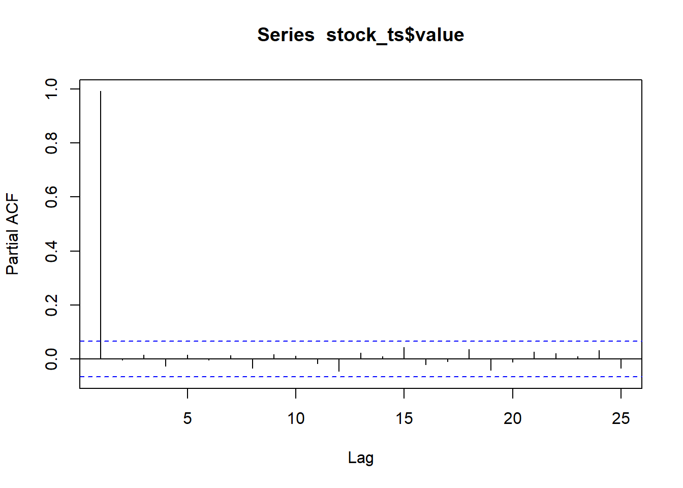

The only significant partial correlation is at lag $k=1$. This suggests that an $AR(1)$ process could be used to model the McDonald’s stock prices.

Partial Autocorrelation Plots of Various $AR(p)$ Processes

Here are some time plots, correlograms, and partial correlograms for $AR(p)$ processes with various values of $p$.

Shiny App

Class Activity: Stationary and Non-Stationary AR Processes (15 min)

Definition of the Characteristic Equation

Treating the symbol $\mathbf{B}$ formally as a number (either real or complex), the polynomial

$${\theta }_p(\mathbf{B})x_t=(1-{\alpha }_1\mathbf{B}-{\alpha }_2{\mathbf{B}}^2-\cdots -{\alpha }_p{\mathbf{B}}^p)x_t$$

is called the characteristic polynomial of an AR process.

If we set the characteristic polynomial to zero, we get the characteristic equation:

$${\theta }_p(\mathbf{B})=(1-{\alpha }_1\mathbf{B}-{\alpha }_2{\mathbf{B}}^2-\cdots -{\alpha }_p{\mathbf{B}}^p)=0$$

The roots of the characteristic polynomial are the values of $\mathbf{B}$ that make the polynomial equal to zero–i.e., the values of $\mathbf{B}$ that make ${\theta }_p(\mathbf{B})=0$. These are also called the solutions of the characteristic equation. The roots of the characteristic polynomial can be real or complex numbers.

We now explore an important result for AR processes that uses the absolute value of complex numbers.

Identifying Stationary Processes

An AR process will be stationary if the absolute value of the solutions of the characteristic equation are all strictly greater than 1.

First, we will find the roots of the characteristic polynomial (i.e. the solutions of the characteristic equation) and then we will determine if the absolute value of these solutions is greater than 1.

We can use the polyroot function to find the roots of polynomials in R. For example, to find the roots of the polynomial $x^2-x-6$, we apply the command

polyroot(c(-6,-1,1))

[1]  3+0i -2+0i

Note the order of the coefficients. They are given in increasing order of the power of $x$.

Of course, we could simply factor the polynomial: $$x^2-x-6=(x-3)(x+2)\stackrel{set}{=}0$$ which implies that $$x=3\text{or}x=-2$$

Definition of the Absolute Value in the Complex Plane

Let $z=a+bi$ be any complex number. It can be represented by the point $(a,b)$ in the complex plane. We define the absolute value of $z$ as the distance from the origin to the point:

$$|z|=\sqrt{a^2+b^2}$$

Practice computing the absolute value of a complex number. $$

Check Your Understanding

Find the absolute value of the following (complex) numbers:

• $-3$

• $4i$

• $-3+4i$

• $-{\displaystyle \frac{\sqrt{3}}{4}}+{\displaystyle \frac{1}{4}}i$

• ${\displaystyle \frac{1}{\sqrt{2}}}-{\displaystyle \frac{1}{\sqrt{2}}}i$

• $5-12i$

We will now practice assessing whether an AR process is stationary using the characteristic equation.

Check Your Understanding

For each of the following AR processes, do the following:

1. Write the AR process in terms of the backward shift operator.
2. Solve the characteristic equation.
3. Determine if the AR process is stationary.

• $AR(1)$ process: $$x_t=x_{t-1}+w_t$$

• $AR(1)$ process: $$x_t=\frac{1}{3}{x}_{t-1}+w_t$$

• $AR(2)$ process: $$x_t=-\frac{1}{4}{x}_{t-1}+\frac{1}{8}{x}_{t-2}+w_t$$

• $AR(2)$ process: $$x_t=-\frac{2}{3}{x}_{t-1}+\frac{1}{3}{x}_{t-2}+w_t$$

• $AR(2)$ process: $$x_t=-x_{t-1}-2x_{t-2}+w_t$$

• $AR(2)$ process: $$x_t=\frac{3}{2}{x}_{t-1}-x_{t-2}+w_t$$

• $AR(2)$ process: $$x_t=4x_{t-2}+w_t$$

• $AR(3)$ process: $$x_t=\frac{2}{3}{x}_{t-1}+\frac{1}{4}{x}_{t-2}-\frac{1}{6}{x}_{t-3}+w_t$$

4. Choose one stationary $AR(2)$ process and one non-stationary $AR(2)$ process. For each, do the following:

• Simulate at least 1000 sequential observations.
• Make a time plot of the simulated values.
• Make a correlogram of the simulated values.
• Plot the partial correlogram of the simulated values.

The following code chunk may be helpful--or you can use the simulation above.

# Number of observations
n_obs <- 1000

# Generate sequence of dates
start_date <- my(paste(1, floor(year(now())-n_obs/365)))
date_seq <- seq(start_date,
    start_date + days(n_obs - 1),
    by = "1 days")

# Simulate random component
w <- rnorm(n_obs)

# Set first few values of x
x <- rep(0, n_obs)
x[1] <- w[1]
x[2] <- 0.6 * x[1] + w[2]

# Set all remaining values of x
for (t in 3:n_obs) {
  x[t] <- 0.6 * x[t-1] + 0.25 * x[t-2] + w[t]
}

# Create the tsibble
sim_ts <- data.frame(dates = date_seq, x = x) |>
  as_tsibble(index = dates) 

# Generate the plots
sim_ts |> autoplot(.vars = x)
acf(sim_ts$x, plot=TRUE, lag.max = 25)
pacf(sim_ts$x, plot=TRUE, lag.max = 25)

5. What do you observe about the difference in the behavior of the stationary and non-stationary processes?

Homework Preview (5 min)

• Review upcoming homework assignment
• Clarify questions

Download Homework

homework_4_3.qmd

Autoregressive Model Definition

Check Your Understanding Solutions

• Show that we can write Equation (4.15) as a polynomial of order $p$ in terms of the backward shift operator: $$(1-{\alpha }_1\mathbf{B}-{\alpha }_2{\mathbf{B}}^2-\cdots -{\alpha }_p{\mathbf{B}}^p)x_t=w_t$$

Solution:

$$x_t={\alpha }_1{x}_{t-1}+{\alpha }_2{x}_{t-2}+{\alpha }_3{x}_{t-3}+\cdots +{\alpha }_{p-1}{x}_{t-(p-1)}+{\alpha }_p{x}_{t-p}+w_t$$ After subtracting, we have: $$\begin{array}{rl}{w}_t& =x_t-{\alpha }_1{x}_{t-1}-{\alpha }_2{x}_{t-2}-{\alpha }_3{x}_{t-3}-\cdots -{\alpha }_{p-1}{x}_{t-(p-1)}-{\alpha }_p{x}_{t-p}\\ & =x_t-{\alpha }_1\mathbf{B}{x}_t-{\alpha }_2{\mathbf{B}}^2{x}_t-{\alpha }_3{\mathbf{B}}^3{x}_t-\cdots -{\alpha }_{p-1}{\mathbf{B}}^{p-1}{x}_t-{\alpha }_p{\mathbf{B}}^p{x}_t\\ & =(1-{\alpha }_1\mathbf{B}-{\alpha }_2{\mathbf{B}}^2-{\alpha }_3{\mathbf{B}}^3-\cdots -{\alpha }_{p-1}{\mathbf{B}}^{p-1}-{\alpha }_p{\mathbf{B}}^p)x_t\end{array}$$

---

• Give another name for an $AR(0)$ model.

Solution:

White noise

---

• Show that the random walk is the special case $AR(1)$ with ${\alpha }_1=1$. (See Chapter 4, Lesson 1.)

Solution:

If we let ${\alpha }_1=1$ in an $AR(1)$ model, we get: $$\begin{array}{rl}{x}_t& ={\alpha }_1{x}_{t-1}+{\alpha }_2{x}_{t-2}+{\alpha }_3{x}_{t-3}+\cdots +{\alpha }_{p-1}{x}_{t-(p-1)}+{\alpha }_p{x}_{t-p}+w_t\\ & ={\alpha }_1{x}_{t-1}+w_t\\ & =x_{t-1}+w_t\end{array}$$ which is the definition of a random walk, as given in Chapter 4, Lesson 1.

---

• Show that the exponential smoothing model is the special case where $${\alpha }_i=\alpha (1-\alpha {)}^i$$ for $i=1,2,\dots$ and $p\to \mathrm{\infty }$. (See Chapter 3, Lesson 2.)

Solution: $$\begin{array}{rl}{x}_t& ={\alpha }_1{x}_{t-1}+{\alpha }_2{x}_{t-2}+{\alpha }_3{x}_{t-3}+\cdots +{\alpha }_{p-1}{x}_{t-(p-1)}+{\alpha }_p{x}_{t-p}+w_t\\ & =\alpha (1-\alpha {)}^1{x}_{t-1}+\alpha (1-\alpha {)}^2{x}_{t-2}+\alpha (1-\alpha {)}^3{x}_{t-3}+\cdots +\alpha (1-\alpha {)}^{p-1}{x}_{t-(p-1)}+\alpha (1-\alpha {)}^p{x}_{t-p}+w_t\end{array}$$

This is Equation (3.18) in Chapter 3, Lesson 2.

---

• Show that the $AR(p)$ model is a regression of $x_t$ on previous terms in the series. (This is why it is called an “autoregressive model.”) Hint: write the $AR(p)$ model in more familiar terms, letting $$y_i=x_t,x_1=x_{t-1},x_2=x_{t-2},\dots ,x_p=x_{t-p},{ϵ}_i=w_t,\text{and}{\beta }_j={\alpha }_j$$

Solution: $$\begin{array}{rl}{x}_t& ={\alpha }_1{x}_{t-1}+{\alpha }_2{x}_{t-2}+{\alpha }_3{x}_{t-3}+\cdots +{\alpha }_{p-1}{x}_{t-(p-1)}+{\alpha }_p{x}_{t-p}+w_t\\ y_i& ={\beta }_1{x}_{1i}+{\beta }_2{x}_{2i}+{\beta }_3{x}_{3i}+\cdots +{\beta }_{p-1,i}{x}_{p-1,i}+{\beta }_p{x}_{p,i}+{ϵ}_i\end{array}$$

This is a multiple linear regression equation with zero intercept.

---

• Explain why the prediction at time $t$ is given by $${\hat{x}}_t={\hat{\alpha }}_1{x}_{t-1}+{\hat{\alpha }}_2{x}_{t-2}+\cdots +{\hat{\alpha }}_{p-1}{x}_{t-(p-1)}+{\hat{\alpha }}_p{x}_{t-p}$$

Solution:

The prediction at time $t$ in a multiple regression setting would be: $${\hat{y}}_i={\hat{\beta }}_1{x}_{1i}+{\hat{\beta }}_2{x}_{2i}+{\hat{\beta }}_3{x}_{3i}+\cdots +{\hat{\beta }}_{p-1}{x}_{p-1,i}+{\hat{\beta }}_p{x}_{p,i}$$ Translated to the $AR(p)$ setting, this becomes: $${\hat{x}}_t={\hat{\alpha }}_1{x}_{t-1}+{\hat{\alpha }}_3{x}_{t-2}+{\hat{\alpha }}_3{x}_{t-3}+\cdots +{\hat{\alpha }}_{p-1}{x}_{t-(p-1)}+{\hat{\alpha }}_p{x}_{t-p}$$

---

• Explain why the model parameters (the $\alpha$’s) can be estimated by minimizing the sum of the squared error terms: $$\sum _{t=1}^n{\left({\hat{w}}_t\right)}^2=\sum _{t=1}^n{(x_t-{\hat{x}}_t)}^2$$

Solution:

This is exactly how the multiple linear regression coefficients are estimated…minimizing the sum of the squared error terms.

---

• What is the reason this is called an autoregressive model?

Solution:

This is called an autoregressive model because we regress the current tern on the previous terms in the series.

Absolute Value

Check Your Understanding Solutions

Find the absolute value of the following (complex) numbers:

• $|-3|=\sqrt{(-3{)}^2+0^2}=3$

• $|4i|=\sqrt{(0{)}^2+(4{)}^2}=4$

• $|-3+4i|=\sqrt{(-3{)}^2+(4{)}^2}=5$

• $|-{\displaystyle \frac{\sqrt{3}}{4}}+{\displaystyle \frac{1}{4}}i|=\sqrt{{\left({\displaystyle \frac{\sqrt{-3}}{4}}\right)}^2+{\left({\displaystyle \frac{1}{4}}\right)}^2}=\sqrt{{\displaystyle \frac{3}{16}}+{\displaystyle \frac{1}{16}}}={\displaystyle \frac{1}{2}}$

• $|{\displaystyle \frac{1}{\sqrt{2}}}-{\displaystyle \frac{1}{\sqrt{2}}}i|=\sqrt{{\left(\frac{1}{\sqrt{2}}\right)}^2+{\left(\frac{-1}{\sqrt{2}}\right)}^2}=1$

• $|5-12i|=\sqrt{(5{)}^2+(-12{)}^2}=13$

Using the Characteristic Polynomial to Assess Stationarity

Check Your Understanding Solutions

For each of the following AR processes, do the following:

1. Write the AR process in terms of the backward shift operator.

2. Solve the characteristic equation.

3. Determine if the AR process is stationary.

• $AR(1)$ process: $$x_t=x_{t-1}+w_t$$

Solution:

---

• $AR(1)$ process: $$x_t=\frac{1}{3}{x}_{t-1}+w_t$$

Solution:

$$\mathbf{B}=3$$ This is a stationary AR process.

---

• $AR(2)$ process: $$x_t=-\frac{1}{4}{x}_{t-1}+\frac{1}{8}{x}_{t-2}+w_t$$

Solution:

$$-\frac{1}{8}({\mathbf{B}}^2-2\mathbf{B}-8)x_t=w_t$$ $$B=-4,B=2$$ This is a stationary AR process.

---

• $AR(2)$ process: $$x_t=-\frac{2}{3}{x}_{t-1}+\frac{1}{3}{x}_{t-2}+w_t$$

Solution:

$$-\frac{1}{3}({\mathbf{B}}^2-2\mathbf{B}-3)x_t=w_t$$ $$B=-1,B=3$$ This is a non-stationary AR process.

---

• $AR(2)$ process: $$x_t=-x_{t-1}-2x_{t-2}+w_t$$

Solution:

$$({\mathbf{B}}^2+1/2\ast \mathbf{B}+1/2)x_t=w_t$$ $$B=\frac{1}{4}\pm \frac{\sqrt{7}}{4}i$$ $$|B|=\sqrt{\frac{1}{16}+\frac{7}{16}i}=\frac{1}{\sqrt{2}}\le 1$$ This is a non-stationary AR process.

---

• $AR(2)$ process: $$x_t=\frac{3}{2}{x}_{t-1}-x_{t-2}+w_t$$

Solution:

$$({\mathbf{B}}^2-\frac{3}{2}\mathbf{B}+1)x_t=w_t$$ $$B=\frac{3}{4}\pm \frac{\sqrt{7}}{4}i$$ $$|B|=1$$ This is a non-stationary AR process.

---

• $AR(2)$ process: $$x_t=4x_{t-2}+w_t$$

Solution:

$$(1-4{\mathbf{B}}^2)x_t=w_t$$ $$B=\pm \frac{1}{2}$$ $$|B|=\frac{1}{2}$$ This is a non-stationary AR process.

---

• $AR(3)$ process: $$x_t=\frac{2}{3}{x}_{t-1}+\frac{1}{4}{x}_{t-2}-\frac{1}{6}{x}_{t-3}+w_t$$

Solution:

$$B=2,-2,\frac{3}{2}$$ This is a stationary AR process.