2-Sample Independent T-Test Practice

Instructions

Here are several opportunities to practice analyzing 2-sample independent t-tests using R. For each question, you will:

Read in data
Identify the Response and Independent variable
Create data summaries (numerical and graphical)
Statistically analyze the data
Check for the suitability of the statistical test (CLT, Normality)
State your hypothesis test conclusions and interpret your confidence intervals

When you finish, render this document and submit the .html in Canvas.

# Load the libraries

library(rio)
library(mosaic)
library(tidyverse)
library(car)

It’s a Date!

Dating Behavior was studied in a speed dating experiment where random matching was generated and created randomization in the number of potential dates. In a survey to each participant, one question was asked about how important attraction is when they date. The attraction value is on a scale from 0 (not important at all) to 100 (very important).

The researchers want to determine if males report to value attractiveness more than females. Use a level of significance of 0.05.

Load the Data

dating <- read_csv('https://github.com/byuistats/Math221D_Course/raw/main/Data/dating_attractive_longformat.csv')

Explore the Data

Question: What is the response variable?
Answer:

Question: What is the explanatory variable?
Answer:

Create a side-by-side boxplot for the amount of reported importance of attractiveness for each biosex.

Add a title and change the colors of the boxes.

What do you observe?

Create a table of summary statistics for each group (favstats()):

Hypothesis Test

State your null and alternative hypotheses (replace the ??? with the appropriate symbol):

\[H_0: \mu_{F}???\mu_{M}\]

\[H_a:\mu_{F}???\mu_{M}\]

NOTE: The default for R is to set group order alphabetically. This means Group 1 = Female.

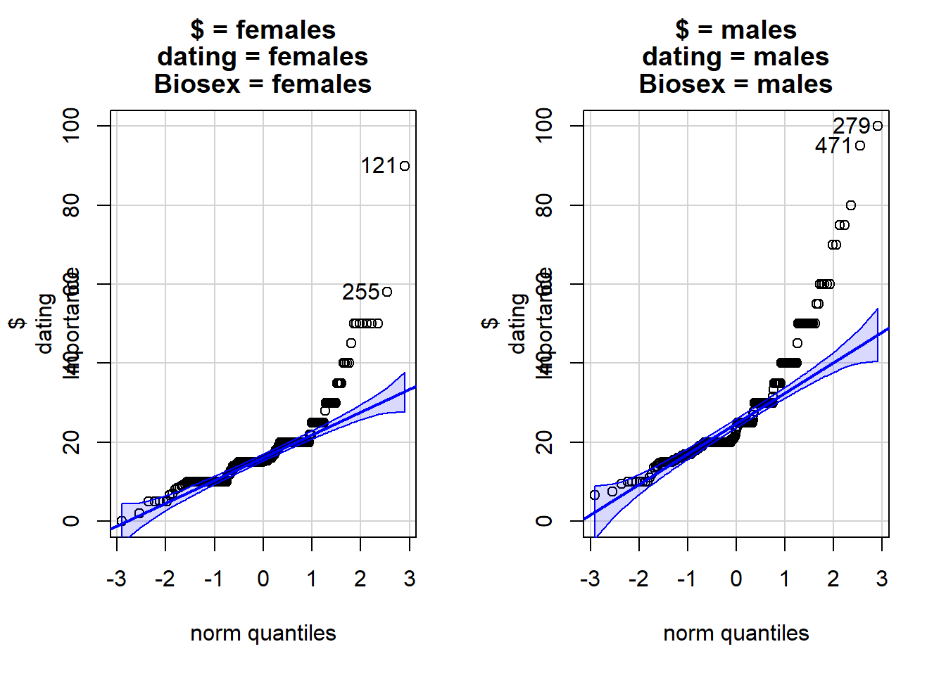
Check that the samples for both groups are normally distributed

qqPlot(dating$Importance~dating$Biosex)

Do the data for each group appear normally distributed?

Why is it OK to continue with the analysis?

Perform a t-test.

Question: What is the value of the test statistic?
Answer:

Question: How many degrees of freedom for this test?
Answer:

Question: What is the p-value?
Answer:

Question: What do you conclude?
Answer:

Confidence Interval

Create a confidence interval for the difference of the average Importance Score between both groups:

Tooth hurty

A simple random sample of dental bill costs was collected at offices in Rexburg and Idaho Falls. Let \(\mu_{IF}\) be the population mean of dental costs in Idaho Falls and \(\mu_{R}\) be the population mean of dentals costs in Rexburg.

We suspect that dental costs are higher in Rexburg because of less competition.

Use the data imported below to answer the following questions.

dentist <- read_csv('https://github.com/byuistats/Math221D_Course/raw/main/Data/DentistOfficeBills_longformat.csv')

Review The Data

Question: What is the response variable?
Answer:

Question: What is the explanatory variable?
Answer:

Create summary statistics tables of dental costs for each office:

Create a side-by-side boxplot for dental costs for each office.

Check the normality of each group.

Question: Do the samples from both groups appear to be normally distributed? If not, is it a cause for concern for our statistical inference?

Hypothesis Test

State your null and alternative hypotheses (replace the question marks with the appropriate symbols):

\[H_0: \mu_{IF}???\mu_{R}\]

\[H_a:\mu_{IF}???\mu_{R}\]

Perform the appropriate analysis:

Question: What is the test statistic?
Answer:

Question: What is the P-value?
Answer:

State your conclusion:

Confidence Interval

Create a confidence interval for the difference in costs between the IF and Rexburg offices:

Explain the confidence interval in context of the research question:

Birth Weights

A study was conducted in which researchers obtained birth weights of infants born in Illinois during the same year. The birth weights are categorized based on the race and birthplace of the mother. Researchers want to know if there is a difference in mean birth weights of babies born to black women who were born in the United States and babies born to black women who were born in Africa. Values were recorded (in grams) for each infant born. The data are recorded in the file.

Let \(\mu_A\) be the population average of babies born to African-born mothers and \(\mu_{IL}\) be the population mean weight of babies born to mothers in Illinois.

Use the data imported below to answer the following questions.

birth_weights <- read_csv('https://github.com/byuistats/Math221D_Course/raw/main/Data/IllinoisBirthWeightsTwoVar_longformat.csv')

Review The Data

Question: What is the response variable?
Answer:

Question: What is the explanatory variable?
Answer:

Create summary statistics tables of birth weights for each country:

Create a side-by-side boxplot for birth weights for each country:

Check the normality of each group.

Question: Do the samples from both groups appear to be normally distributed? If not, is it a cause for concern for our statistical inference?

Hypothesis Test

State your null and alternative hypotheses (replace the question marks with the appropriate symbols):

\[H_0: \mu_{A}???\mu_{IL}\]

\[H_a:\mu_{A}???\mu_{IL}\]

Perform the appropriate analysis:

Question: What is the test statistic?
Answer:

Question: What is the P-value?
Answer:

State your conclusion:

Confidence Interval

Create a confidence interval for the average difference in weights between babies born to mothers in Africa and Illinois:

Explain the confidence interval in context of the research question:

Miscellany

Question: A financial economist is studying married couples in which both spouses work. He wants to compare the mean income earned by husbands with the mean income earned by their wives. Should he use independent sampling or dependent sampling, and why?
Answer: