# Load Libraries

library(tidyverse)
library(mosaic)
library(rio)
library(car)


# Load Data
big5 <- import('https://raw.githubusercontent.com/byuistats/Math221D_Cannon/master/Data/All_class_combined_personality_data.csv')Don’t Take it Personally
Hypothesis Tests and Confidence Intervals
Introduction
In this activity, you will execute statistical hypothesis tests and generate confidence intervals for each of the Big 5 personality traits using data collected from a random sample of Brother Cannon’s Math 221 students.
Question: What is the population of this analysis?
Answer:
For each personality trait, include:
- A statement of the null and alternative hypotheses and why you chose the alternative you did.
- Choose alpha, $= $
- Check that you can trust the normality of the mean (
n > 30orqqPlot(respons_variable)) - Run the one-sample t-test and state your conclusion (technical and contextual explanation)
- Calculate a
Recall that we can use favstats() to get summary statistics, boxplot() and histogram() to get visualizations, and the t.test() function to get hypothesis tests and confidence intervals. Be sure to label your plots’ axes and include a title.
Extroversion
State your null and alternative hypotheses:
1. Create a table of summary statistics:
# Extroversion

favstats(big5$Extroversion) %>% knitr::kable()| min | Q1 | median | Q3 | max | mean | sd | n | missing | |
|---|---|---|---|---|---|---|---|---|---|
| 1 | 42 | 58 | 73 | 100 | 56.98267 | 21.09599 | 404 | 1 |
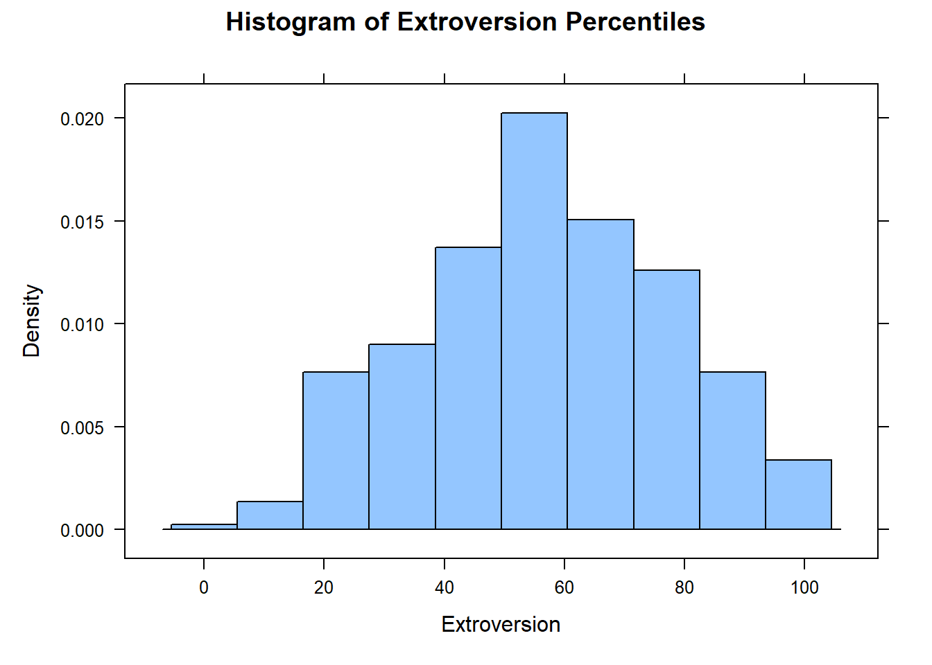
- Create a histogram of Extroversion:
### I'm making a single variable called "extrov" that drops the missing values.  You can do the same thing with the other traits to make analysis a little easier
extrov <- na.omit(big5$Extroversion)

histogram(extrov, xlab = "Extroversion", main = "Histogram of Extroversion Percentiles")
- Perform the one-sample t.test:
# For Hypothesis Test:
t.test(extrov, mu = 50, alternative = "greater")
    One Sample t-test

data:  extrov
t = 6.6529, df = 403, p-value = 4.697e-11
alternative hypothesis: true mean is greater than 50
95 percent confidence interval:
 55.25232      Inf
sample estimates:
mean of x
56.98267 - Explain your conclusion:
Technical: Because the p-value is less than
Contextual: I have sufficient evidence to suggest that Brother Cannon’s students are, on average, more Extroverted than the general population.
- Create a Confidence Interval for the average extroversion of Brother Cannon’s students:
# For a Confidence Interval:
t.test(extrov, conf.level = 1-.025)$conf.int
[1] 54.62135 59.34399
attr(,"conf.level")
[1] 0.975- Explain your confidence interval:
I am 97.5% confident that the true average extroversion of Brother Cannon’s students is somewhere between the 54.62 and 59.34 percentiles.
Agreeableness
State your null and alternative hypotheses. For example, do you think Brother Cannon’s students are more, less, or just different than the general population?
1. Create a table of summary statistics for Agreeableness:
- Create a histogram of Agreeableness:
- Perform the one-sample t.test:
- Explain your conclusion:
Technical:
Contextual:
- Create a Confidence Interval for the average agreeableness of Brother Cannon’s students:
# For a Confidence Interval:
t.test()$conf.int
Error in t_test.default(): argument "x" is missing, with no default- Explain your confidence interval:
Openness
State your null and alternative hypotheses:
- Create a table of summary statistics for Openness:
- Create a histogram of Openness:
- Perform the one-sample t.test:
- Explain your conclusion:
Technical:
Contextual:
- Create a Confidence Interval for the average openness of Brother Cannon’s students:
# For a Confidence Interval:
t.test()$conf.int
Error in t_test.default(): argument "x" is missing, with no default- Explain your confidence interval:
Neuroticism
State your null and alternative hypotheses:
1. Create a table of summary statistics for Neuroticism:
- Create a histogram of Neuroticism:
- Perform the one-sample t.test:
- Explain your conclusion:
Technical:
Contextual:
- Create a Confidence Interval for the average neuroticism of Brother Cannon’s students:
# For a Confidence Interval:
t.test()$conf.int
Error in t_test.default(): argument "x" is missing, with no default- Explain your confidence interval:
Conscientiousness
State your null and alternative hypotheses:
1. Create a table of summary statistics:
- Create a histogram of Conscientiousness:
- Perform the one-sample t.test:
- Explain your conclusion:
Technical:
Contextual:
- Create a Confidence Interval for the average conscientiousness of Brother Cannon’s students:
# For a Confidence Interval:
t.test()$conf.int
Error in t_test.default(): argument "x" is missing, with no default- Explain your confidence interval: