Inference for a Mean - Sigma Unknown

One-Sample T-test and Confidence Intervals

Lesson Objectives

By the end of this lesson, you should be able to:

Recognize when a one mean (sigma unknown) inferential procedure is appropriate
Perform a hypothesis test for one mean (sigma unknown) using the following steps:
1. State the null and alternative hypotheses
2. Calculate the test-statistic, degrees of freedom and P-value using R
3. Assess statistical significance in order to state the conclusion for the hypothesis test in context of the research question
4. Check the requirements for the hypothesis test
Create a confidence interval for one mean (sigma unknown) using the following steps:
1. Calculate a confidence interval for a given level of confidence using R
2. Interpret the confidence interval
3. Check the requirements of the confidence interval
State the properties of the Student’s t-distribution

Review

When we know what the population standard deviation, $σ$ , for individuals, and are confident that the distribution of sample means is approximately normal, we can use a Z-score and the Standard Normal Distribution to calculate probabilities.

$z = \frac{\bar{x} - μ}{\frac{σ}{\sqrt{n}}}$

Though rare, there are situations where we might know the population standard deviation from published research or census data. For example, standardized test organizations publish population-level summaries which would allow us to test how our sample compares to the general population using the Z formula.

Confidence Interval

We can also calculate a confidence interval for the above example.

Recall the formula for a confidence interval is, for a given $z^{*}$ associated with a desired level of confidence:

$C I = \bar{x} \pm z^{*} \frac{σ}{\sqrt{n}}$

Recall the $z^{*}$ for common confidence levels:

library(tidyverse)
library(pander)
tibble(`Conf. Level` = c(0.99, 0.95, 0.90), `Z*` = c(2.576, 1.96, 1.645)) %>% pander()

Conf. Level	Z*
0.99	2.576
0.95	1.96
0.9	1.645

Student’s T-Distribution (sigma unkown)

In most cases, we perform statistical analyses on samples from a population where we don’t know the population standard deviation, $σ$ .

A simple solution is to use the sample standard deviation, $s$ , instead of $σ$ . We calculate test statistics very similarly to a Z-score.

$t = \frac{\bar{x} - μ}{\frac{s}{\sqrt{n}}}$

Unfortunately, the above test statistic is not a standard normal distribution. W can no longer use pnorm() to calculate probabilities because the distribution of $t$ is not normal.

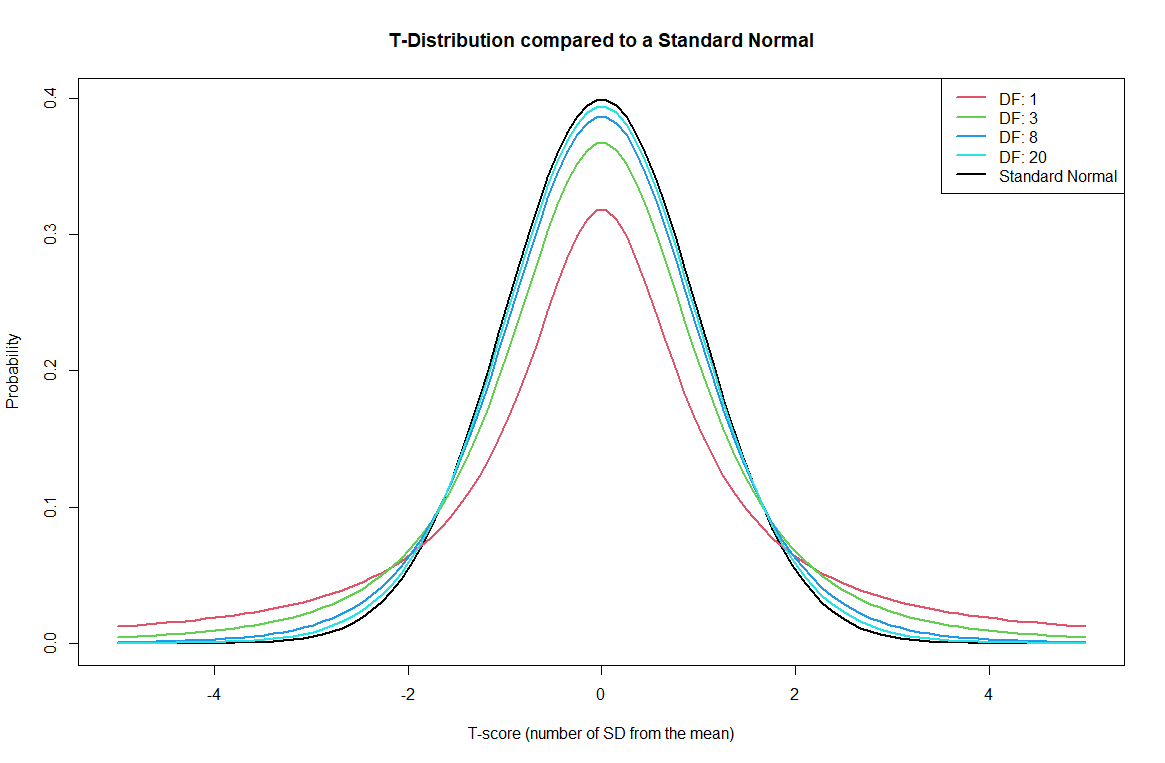
We use a distribution that is similar to the Normal distribution but whose shape depends on how much data we have. The Student’s t-distribution requires a t-value (like a z-score) and something called degrees of freedom.

Degrees of Freedom for a t-distribution are defined:

$d f = n - 1$

The T-distribution is very similar to the standard normal. It is symmetrical around zero. However, the shape depends on how much data you have. The more data you have, the closer the $t$ is to the standard normal. This is illustrated in the graph below:

Even though $t$ is not normally distributed, R is fully capable of calculating probabilities for many probability distributions including the t-distribution. We can use the pt() function which requires a t-value and degrees of freedom.

Calculating P-values by hand with the T-distribution (One out of ten. Would NOT RECOMMENDED)

Suppose we have 25 test scores defined as “data” in the code chunk below. We can calculate the $t$ -statistic just like we did with the $z$ -score.

Suppose we believe that the mean score of these 25 students is significantly higher than 50. Our null and alternative hypothesis are as follows:

$H_{0} : μ = 50$ $H_{a} : μ > 50$

# we can use the t-distribution, pt(), just like pnorm() but must also add the degrees of freedom

data <- c(88,81,27,92,46,79,67,44,46,88,21,60,71,81,79,52,100,44,42,58,52,48,83,65,98)

# Hypothesized Mean:
mu_0 <- 50

# Sample size, sample Mean and sample SD
#  The length function tells us how many data points are in the list.  
n <- length(data)
xbar <- mean(data)
s <- sd(data)

s_xbar = s / sqrt(n)

t <- (xbar - mu_0) / s_xbar

# Probability of getting a test statistic at least as extreme as the one we observed if the null hypothesis is true
1-pt(t, n-1)

[1] 0.00151866

This means that if the true population mean was 50, then there is only a 0.00152 probability of observing a test statistic, t, as high as the one we got (P-value).

The Easy Way

The good news is that the more complicated the math becomes, the less of it we have to do! Instead of using R like a calculator to calculate $z$ or $t$ -scores and calculating probabilities “by hand” (using pnorm() or pt()), we can use R functions with the data directly and get much more useful output.

For situations where we want to make inference about a population from our sample data, we will be following these basic steps:

Read in the data
Review the data
Visualize the data
Perform the appropriate analysis

This will be true regardless of the type of data and analysis. Let’s begin by looking at a familiar dataset. In the following example, we will focus on the Extroversion scores from Brother Cannon’s Math 221 classes.

Step 1: Read in the data

# Load Libraries

library(tidyverse)
library(mosaic)
library(rio)
library(car)


# Read in data
big5 <- import('https://raw.githubusercontent.com/byuistats/Math221D_Cannon/master/Data/All_class_combined_personality_data.csv')

Step 2: Review the Data

In this step, we are looking to see if the data are as expected. Are the columns we’re interested in numeric? Categorical? and do these match expectations. We can also start to look for strange data and outliers. Visualizations can help.

Other common issues to look for include: negative numbers that should only be positive, date values that shouldn’t exist, missing values, character variables inside what should be a number.

In the real world, data are messy. Reviewing the data is a critical part of an analysis.

Take a look through the personality dataset and see if there are any anomalies that might need to be addressed.

Step 3: Visulize the data

So far we have been discussing a single, quantitative variable of interest, like test scores, reaction times, heights, etc. When we start looking at more complicated data, we will expand our repertoire of visualizations, but Histograms are very good when looking at one variable at a time, and boxplots are very good for comparison between groups.

Create a histogram of Extroversion. Describe some features of the data. Is it symmetric? Skewed? Are there outliers?

histogram(big5$Extroversion, main = "Extroversion Scores", xlab = "Extroversion")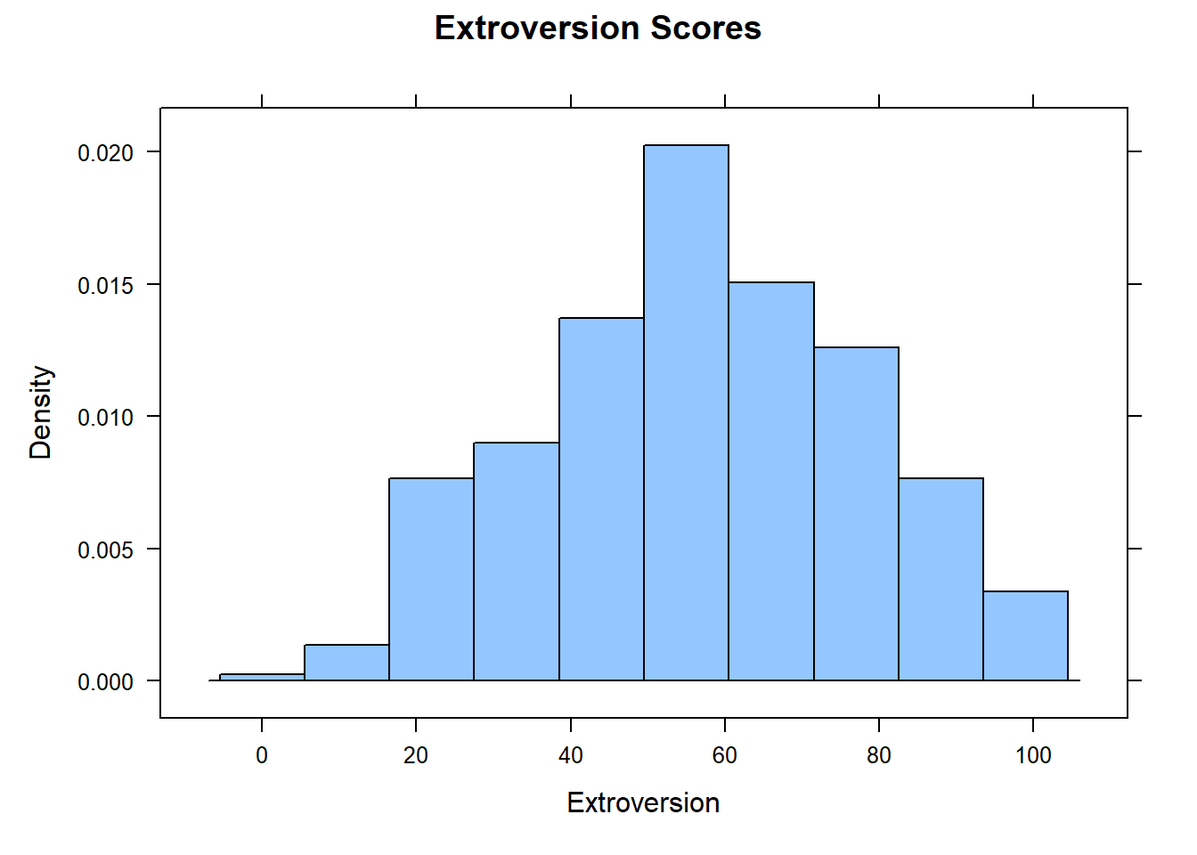

ggplot(big5, aes(x = Extroversion)) +
  geom_histogram(bins = 15, fill="lightblue") +
  labs(
    x = "Extroversion",
    y = "",
    title = "Extroversion Scores"
  ) +
  theme_bw()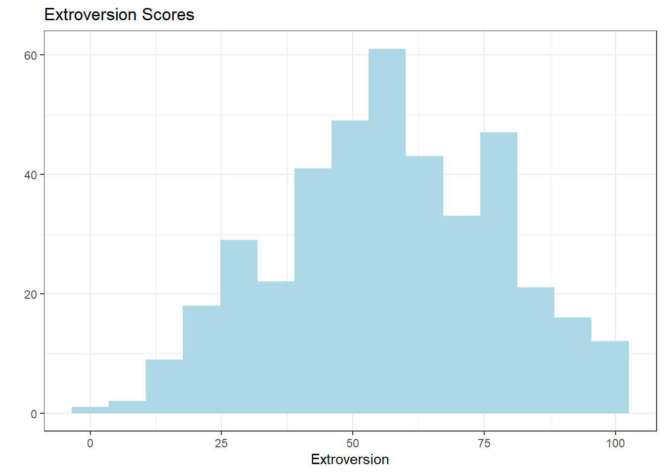

Step 4: Perform the appropriate analysis

In this example, we will be testing the hypothesis that Brother Cannon’s students are similar to the general population. We suspect that these youthful BYU-I students are, on average, more extroverted.

Hypothesis Test

Write out the Null and alternative hypotheses.

$H_{0} : μ_{e x t r o v e r s i o n} = 50$

$H_{A} : μ_{e x t r o v e r s i o n} > 50$

$α = 0.05$

Perform the one-sample t-test using the “t.test()” function in R. If you ever get stuck remembering how to use a function in R, you can run ?t.test to see documentation. The question mark will open up the help files for any given function in R.

The t.test() function takes as input, the data, the hypothesized mean, mu, and the direction of the alternative hypothesis.

The default parameters for the t.test() function are: t.test(data, mu = 0, alternative = "two.sided").

#?t.test

# One-sided Hypothesis Test
t.test(big5$Extroversion, mu = 50, alternative = "greater")


    One Sample t-test

data:  big5$Extroversion
t = 6.6529, df = 403, p-value = 4.697e-11
alternative hypothesis: true mean is greater than 50
95 percent confidence interval:
 55.25232      Inf
sample estimates:
mean of x 
 56.98267

Question: What is the P-value?
Answer: p-value = 4.697e-11

QUESTION: What is your conclusion based on $α = 0.05$ ?
ANSWER: Because P-value < 0.05 we reject the null hypothesis in favor of the alternative.

Question: State your conclusion in context of our research question?
Answer: We have sufficient evidence to conclude that Brother Cannon’s students are more extroverted than the general population, on average.

Confidence Intervals

We can also use the t.test() function to create confidence intervals. Recall that confidence intervals are always 2-tailed. Confidence intervals are typically written in the form: (lower limit, upper limit).

# Confidence Intervals are by definition 2-tailed
# We can also change the confidence level

t.test(big5$Extroversion, mu = 50, alternative = "two.sided", conf.level = .99)


    One Sample t-test

data:  big5$Extroversion
t = 6.6529, df = 403, p-value = 9.394e-11
alternative hypothesis: true mean is not equal to 50
99 percent confidence interval:
 54.26631 59.69903
sample estimates:
mean of x 
 56.98267

To get only the output for the confidence interval to be shown, we can use a $ to select specific output. Much like when pulling a specific column from a dataset, the $ can pull specific output from an analysis.

Because the option for the alternative = in the t.test function is “two.sided”, we don’t actually need to include it when getting confidence intervals.

Also, confidence intervals do not require an assumed mu value. So a more efficient way to get a confidence interval for a given set of data is:

t.test(big5$Extroversion, conf.level = .99)$conf.int

[1] 54.26631 59.69903
attr(,"conf.level")
[1] 0.99

Question: Describe in words the interpretation of the confidence interval in context of Extroversion.
Answer: I am 95% confident that the true population mean of extroversion scores for Brother Cannon’s students is between 54.266 and 59.699.

Checking Requirements

We still rely on the assumption that the distribution of sample means is normally distributed.

Recall that the mean is normally distributed if:

The underlying population is normally distributed
We have a sufficiently large sample size ( $n > 30$ )

For the above Extroversion data, we have $n = 404$ which is much larger than 40.

If my sample size was small, I could check the qqPlot(), which I demonstrate here:

qqPlot(big5$Extroversion)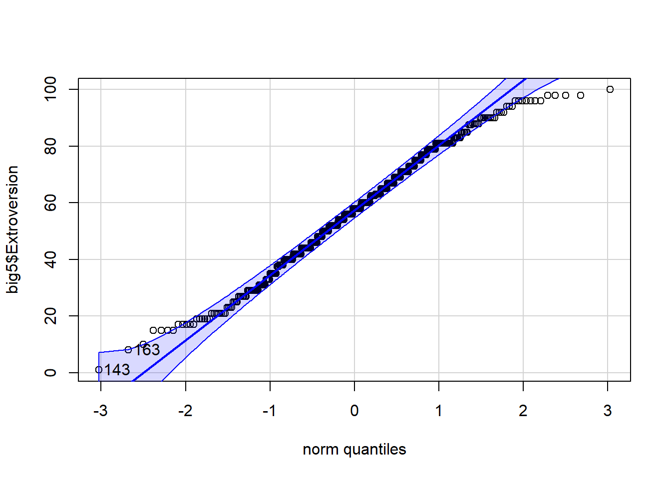

[1] 143 163

Your Turn

Body Temperature Data

The dataset below contains information about body temperatures of healthy adults.

Load the data:

# These lines load the data into the data frame body_temp:

body_temp <- import("https://byuistats.github.io/M221R/Data/body_temp.xlsx")

Review the Data

Create a table of summary statistics for temperature:

Visualize the Data

Create a histogram to visualize the body temperature data.

Question: Describe the general shape of the distribution.
Answer:

Analyze the Data

It’s widely accepted that normal body temperature for healthy adults is 98.6 degrees Fahrenheit.

Suppose we suspect that the average temperature is different than 98.6

Use a significance level of $α = 0.01$ to test whether the mean body temperature of healthy adults is equal to 98.6 degrees Fahrenheit.

Question: What is the P-value?
Answer:

QUESTION: What is your conclusion?
ANSWER:

Confidence Interval

Create a 99% confidence interval for the true population average temperature of healthy adults.

Check the requirements for the t-test ( $n > 30$ or qqPlot()):

QUESTION: Are the requirements for the t-test satisfied?
ANSWER: