This lesson explores the idea of a sampling distribution which is the theoretical distribution of a sample statistic. We discuss the theoretical concepts that allow us to make confident conclusions about an entire population based on a single sample.
Lesson Outcomes
By the end of this lesson, you should be able to:
Describe the concept of a sampling distribution of the sample mean
State the Central Limit Theorem
Determine the mean of the sampling distribution for a given parent population
Determine the standard deviation of the sampling distribution of the sample mean for a given parent population
Determine the shape of the sampling distribution of the sample mean for a given parent population
State the Law of Large Numbers
Review
A Population Parameter is a numerical summary (mean, median, standard deviation, proportion, etc.) based on the entire population.
A Sample Statistic is any numerical summary (mean, median, standard deviation, proportion, etc.) based on a sample from a population.
A Sample is a subset of the entire population.
Sample Size is the number of individuals in the sample.
Randomization is used in the collection of a sample to minimize bias and make sure our sample is representative of the population.
The Consequences of Randomization
Randomization guarantees that if someone else tries to recreate our study, they will get a different sample. Consequently, their sample statistics will not be the same as ours!
While this should not be surprising, it does create a problem. Given sample-to-sample differences, how can we know when our conclusions are valid? We typically only have one sample to go on.
The good news is that we can rely on the theory of sampling distributions to quantify the uncertainty about our sample.
Sampling Distributions
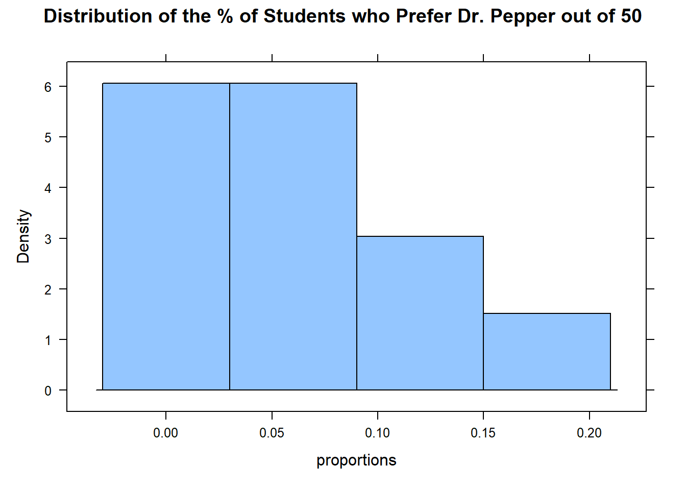
Imagine you and 10 friends want to know about the what percent of BYU-I students whose favorite soda is Dr. Pepper. Each of you could go and survey 50 people each and ask about their favorite soda. All 11 of you calculate the proportion of students who prefer Dr. Pepper.
You’ll all get different results because you’ll be asking different sets of people. Now, instead of looking at your percents individually, summarize the collection of samples from all 11 of you using favstats() and a histogram:
histogram(proportions, main ="Distribution of the % of Students who Prefer Dr. Pepper out of 50")
The above histogram represents 11 different samples of nearly infinite possible samples of 50 BYU-I students.
The Sampling Distribution is the distribution of a sample statistic for all possible samples from a population. It’s completely theoretical, but there are some mathematically provable attributes of this theoretical distribution that make it possible to make inference about an unknown population parameter based on a single sample.
We will discuss these theoretical properties in greater detail below. Before we do, use your intuition to answer the following question.
Answer the following question:
QUESTION: Given the 11 independent samples of 50 students, what would be your best guess of the True population proportion of students who prefer Dr. Pepper?
NOTE: Because these results are based on a simulation, the true proportion is known.
Show/Hide Solution
If you guessed the mean of the 11 samples (0.0709) you’d be VERY close to the truth, which is 7%. Even though none of the individual researchers got 7%, their average was close to the truth! (It’s actually impossible to get exactly 7% when only asking 50 students.)
It turns out that the mean of the sampling distribution of a sample statistic is equal to the population parameter!
The Central Limit Theorem allows us to know not only know about the mean, but the entire shape of the sampling distribution for a mean.
The Central Limit Theorem
For any population with a mean, , and a standard deviation, :
The Central Limit Theorem states that with a sufficiently large sample size, the sampling distribution of the sample mean will be approximately normal with a mean equal to the population mean, , and a standard deviation equal to the population standard deviation, where is the number of individuals in the sample.
When is Normal?
How many observations are required so that the Central Limit Theorem will assure that the distribution of sample means will be approximately normal? The answer is, “it depends.”
If the parent population is normal, then the sampling distribution of will always be normally distributed, no matter how many observations are selected.
If the parent population is not normal, then the sampling distribution will be approximately normally distributed, if the sample size is large enough.
If the parent population is almost normal (e.g. mound-shaped and nearly symmetrical), then a sample of size n = 5 will probably be sufficient to assure that will be approximately normally distributed.
If the parent population is heavily skewed, then it will require a larger sample size to be assured that will be normally distributed. For most moderately skewed distributions, a sample size of around 30 is traditionally thought to be sufficiently large to assure that will be approximately normally distributed. This is not a definitive number but is a rule of thumb.
For tremendously skewed distributions (e.g., the distribution of lottery payouts), a much larger sample will be required before the distribution of sample means is approximately normal. This may require billions of observations. Simulation can be used to determine if a particular sample size is sufficient.
For this course, if the sample size is at least 30, we will conclude that the sampling distribution of will be approximately normal.
Answer the following question:
There are two ways that can be (approximately) normally distributed. What are they?
Show/Hide Solution
will be normally distributed if the data were drawn from a normal population.
will be approximately normally distributed if the sample size is sufficiently large.
Mean and Standard Deviation of the Distribution of Sample Means
The following facts are always true. They do not depend on the Central Limit Theorem. They do not depend on the sample size. These facts hold for the sample mean of any simple random sample of size drawn from a population with mean and standard deviation .
The mean of the sample means is
The standard deviation of the sample means is
Remember, these facts are always true. They do not depend on normality or the sample size. So, even though these facts are often used in conjunction with the Central Limit Theorem, they do not depend on it.
Think about the simulations you have observed. The mean of the sample means was always aligned with . Also, if you took samples larger than , the standard deviation of sample means was always smaller than .
Answer the following questions:
The amount of time passengers spend waiting for a bus on a particular urban route follows a distribution that has a mean of 8.7 minutes with a standard deviation of 2.2 minutes. Transportation officials observed the waiting times for a random sample of individual passengers and recorded the sample mean, . We can think of this sample mean as one value observed out of all the possible sample means that could have been observed. What is the mean of the distribution of all possible sample means?
Show/Hide Solution
Use the information in the previous problem to answer this question: What is the standard deviation of the distribution of all possible sample means?
Show/Hide Solution
The Law of Large Numbers
Suppose researchers treated 6 patients with a new cancer treatment. Their estimated 5-year survival rate was estimated to be 50% higher than standard treatment. How confident would you be in my results?
While it is possible that the new treatment is wildly more effective than standard treatments, six patients is not a lot. It is possible to get six patients that might be more resilient than average, just by chance. Six people can hardly be a robust, representative of the whole population.
My sample mean survival rate is not likely to be very close to the true population survival rate.
The Law of Large Numbers states that the sample mean, , will become closer to as the sample size becomes larger.
Answer the following questions:
We just learned that the standard deviation of sample means is . What happens to the standard deviation of sample means when the sample size is increased?
Show/Hide Solution
If the sample size, , is increased, then the standard deviation of the sample mean will decrease. The fraction will get smaller.
If the standard deviation of the sample mean gets smaller, what happens to the values of ?
Show/Hide Solution
The values that will be observed will be very close to each other and therefore close to , if the sample size is large.
The result you have discovered in the previous two questions is called the Law of Large Numbers. The Law of Large Numbers states that if the sample size is large, then the sample mean will typically be close to the population mean, . This happens because the standard deviation will get smaller as the sample size increases.
NOTE: This is very different from the Central Limit Theorem. The Central Limit Theorem is a statement about the DISTRIBUTION of all possible sample means, that if the sample size is large that will be approximately normal. The Law of Large numbers states that the sample mean will be close to .
Take a moment to study the difference between the Central Limit Theorem and the Law of Large Numbers. They are very different, but it is easy to mix them up when you are first learning about them.
Review of Key Concepts
In order to “do statistics” we need to compute probabilities. This requires we know the distribution of the population of interest. The most important distribution in this course is the normal distribution. In this lesson, we are interested in another very important distribution: the distribution of all the sample means, . In order to do statistics with we need the sampling distribution of to be normal. There are two situations when the distribution of is guaranteed to be normal (or at least very close to normal). They are:
If the parent population is normal, the distribution of the sample means will be normal, for every sample size .
Even if the parent population is not normal, the Central Limit Theorem guarantees that the distribution of the sample mean will be approximately normal if the sample size is large enough. For this course, if, we will say the distribution of the sample means will be approximately normal (even if the parent population is not normal).
The mean and standard deviation of are:
The mean of the sample means is the population mean .
The standard deviation of the sample means is the population standard deviation divided by the square root of ,
Summary
Remember…
The distribution of sample means is a distribution of all possible sample means () for a particular sample size.
The Central Limit Theorem states that the sampling distribution of the sample mean will be approximately normal if the sample size of a sample is sufficiently large. In this class, is considered to be sufficiently large.
The mean of the distribution of sample means is the mean of the population: .
The standard deviation of the distribution of sample means is the standard deviation of the population divided by the square root of : .
The distribution of sample means is normal in either of two situations: (1) when the data is normally distributed or (2) when, thanks to the Central Limit Theorem (CLT), our sample size () is large.
The Law of Large Numbers states that as the sample size () gets larger, the sample mean () will get closer to the population mean (). This can be seen in the equation for . Notice as increases, then will get smaller.