Inference for a Mean

Hypothesis Testing and Confidence Intervals

Introduction

Statistical Inference is the practice of using data sampled from a population to make conclusions about population parameters.

The two primary methods of statistical inference are:

1. Hypothesis Testing
2. Confidence Intervals

Hypothesis testing is the practice of gathering evidence in an attempt to disprove a hypothesis. We either reject the conventional wisdom or fail to reject it.

Confidence intervals are a way to use data to estimate the unknown population parameter, often the population mean, $\mu$.

This chapter lays the foundation for Hypothesis Testing.

Review: distribution of sample means

Hypothesis testing depends on the validity of the assumption that the distribution of the sample mean is normally distributed.

Recall that the distribution of sample means is normal when:

1. The underlying population is normally distributed
2. The sample size, n, is sufficiently large ($n<30$ for this class) for the Central Limit Theorem to apply

Hypothesis Testing

When we know the population standard deviation, $\sigma$, for individuals, we calculate Z-scores and used the Standard Normal Distribution to calculate probabilities. Z has what is called a standard normal distribution, meaning it has a mean of 0 and a standard deviation of 1.

$$z=\frac{\overline{x}-\mu }{\frac{\sigma }{\sqrt{n}}}$$

NOTE: In practice, we do not typically know the population standard deviation. To help us make the connection between probability calculations for means and hypothesis testing, we assume we know the population standard deviation, $\sigma$.

Testing fo the True Mean Length of a Footlong Sandwich

One might expect a foot-long sandwich to be 12 inches long, at least on average. Consumers will naturally allow for some level of variation. But if enough customers are convinced they are getting consistently short-changed, they may loudly complain, or even attempt a lawsuit.

The Null Hypothesis

Proper scientific inquiry is based on attempts to disprove a claim. The claim representing the “status quo,” the commonly held belief or the usual value is called the null hypothesis. In the case of foot-long sandwiches, our null hypothesis is that the true mean length of foot-long sandwiches is 12 inches.

We present the null hypothesis in the following way:

$$H_0:\mu =12$$ We label the null hypothesis $H_0$, often pronounced “H-nought”. The zero in the subscript represents “null,” “baseline,” “default,” “no effect,” etc.

The null hypothesis is standing trial. We seek evidence against $H_0$ in favor of an alternative.

The Alternative Hypothesis

The alternative hypothesis, $H_a$, is the proposed challenge to $H_0$. In the case of foot-long sandwiches, customers will typically only get upset if they are getting less than advertised. We would propose an alternative:

$$H_a:\mu <12$$

There are other possible alternatives that will depend on the context of the research question. Sometimes we may want to test if something is higher than a proposed value. Sometimes we are not sure if something is higher or lower at the outset, so we could test if something is not equal to a proposed value.

Alternative hypothesis could have been written as:

• $H_a:\mu \ne 12$ (two-sided hypothesis; two-tailed)
• $H_a:\mu <12$ (one-sided hypothesis; left-tailed)
• $H_a:\mu >12$ (one-sided hypothesis; right-tailed)

It is important that the null and alternative hypotheses be determined prior to collecting the data. It is not appropriate to use the data from your study to choose the alternative hypothesis that will be used to test the same data! This is an example of using data twice, once to choose the test and again to conduct the test. It is okay to use data from a previous study to determine your null and alternative hypotheses, but it is an improper use of the statistical procedures to use the data to define and conduct a hypothesis test.

KEY POINTS:

1. Hypotheses are statements about population parameters
2. The null hypothesis will always be a statement of equality
3. We never PROVE the null hypothesis is true, we can only fail to disprove it.

That last point is important. Data collected are only evidence against $H_0$. This is similar to the situation in a courtroom where a defendant is accused of a crime. The defendant does not have to PROVE their innocence. It is up to the prosecution to prove guilt. If they fail to do so, we find the defendant “not guilty”, which is not the same thing as innocent. It just means there wasn’t enough evidence to convict.

Test Statistic

We use Test Statistics to determine how likely our results are assuming the null hypothesis is true. We will use many different test statistics throughout this course, but the first one will be very familiar: the Z-score.

When testing a null hypothesis, the $\mu$ in the z-score formula becomes the hypothesized population mean. The $z$-score is then interpreted as the number of standard deviations away from the hypothesized mean. If we know the population standard deviation, $\sigma$, then we can calculate the probability of getting a sample mean more extreme than the one we observed if the null hypothesis is true.

Suppose for now that sandwich-to-sandwich lengths vary by about 0.5 inches and that the distribution is normal. If we sampled 21 random sandwiches from shops in a region and got a sample mean length of 11.82 inches, we can calculate a Z-score:

$$z=\frac{\overline{x}-{\mu }_0}{\sigma /\sqrt{n}}=\frac{11.82-12}{0.5/\sqrt{21}}=-1.649727$$

Where $z$ is the test statistic, $\overline{x}$ is the sample mean, ${\mu }_0$ is the null hypothesis mean, $\sigma$ is the population standard deviation and $n$ is the sample size.

Based on the results from the formula above, $\overline{x}$ is about 1.65 standard deviations below the mean.

We can then use this Z-score to calculate the probability of observing such a result or more extreme, if the null hypothesis is true. This is the evidence we are going to use to make a decision about the null hypothesis.

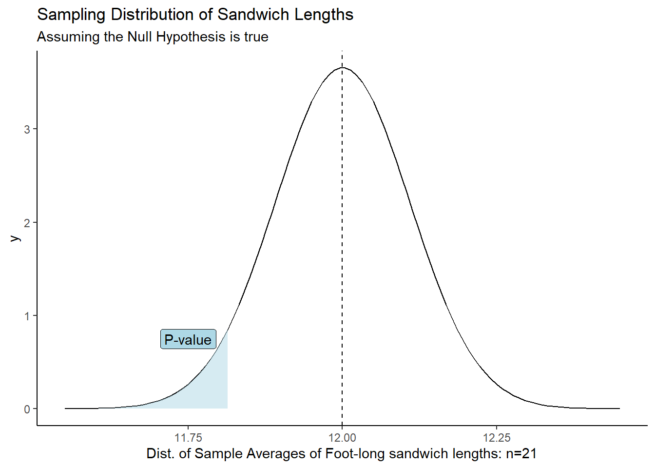
$P$-value

$P$-value: The probability of obtaining a test statistic (such as $z$) at least as extreme as the one you calculated, assuming the null hypothesis is true.

In other words, our $P$-value is the probability that we would get a $z$-score that is as extreme or more extreme than $z=-1.649727$, assuming the true mean is 12 inches.

KEY DEFINITION: A P-value is the probability of observing a test statistic as extreme, or more extreme than the one we observed in our sample, if the null hypothesis is true.

We use “as or more extreme” because the direction (greater than or less than) depends on our alternative hypothesis.

In the case against the sandwich shop, we can use pnorm() to get the P-value:

z <- (11.82-12) / (0.5/sqrt(21))

pnorm(z)

[1] 0.04949937

Conclusion: If the true population mean was 12 inches, there is a 4.95% chance of obtaining a sample mean of 11.82 hours for a sample of size 21.

At this point we have to make a decision. Is that probability small enough to reject the null hypothesis in favor the alternative? Are foot-long sandwich is LESS than 12 inches on average?

When the P-value is very small, we have strong evidence to reject the null hypothesis. But how small is small enough?

Level of Significance, $\alpha$

We need a number that can be used to determine if the $P$-value is small enough to reject the null hypothesis that is not dependent on the data. This number is called the level of significance and is often denoted by the symbol $\alpha$ (pronounced “alpha”.)

We will use the same decision rule for all hypothesis tests:

1. If the $P$-value is less than $\alpha$, we reject the null hypothesis.
2. If the $P$-value is greater than $\alpha$, we fail to reject the null hypothesis.

Memory Aid: Some students find it helpful to remember the decision rule using the couplet:

If $P$ is low, reject $H_O$

Where “low” means less than $\alpha$.

The level of significance, $\alpha$, must be chosen prior to collecting the data. If we wanted to reject the null hypothesis, we could compute the $P$-value and then unscrupulously choose the $\alpha$ level. In every case, we could choose a value of $\alpha$ that is larger than the computed $P$-value, and therefore always reject the null hypothesis. This practice would defeat the purpose of hypothesis testing.

Type I and Type II Errors

This is not an infallible process. We may end up rejecting a null hypothesis that is, in fact, true. Or fail to reject a null hypothesis that is, in fact, false.

This is because researchers will sometimes get a very high or very low sample mean purely by chance. Perhaps their sampling methods were not as random as they had supposed. We may reject or fail to reject a null hypothesis because of dumb luck.

Type I Error: Rejecting a TRUE null hypothesis.

Assuming the null hypothesis is true, the level of significance ($\alpha$) is the probability of getting a value of the test statistic that is extreme enough that the null hypothesis will be rejected. In other words, the level of significance ($\alpha$) is the probability of committing a Type I error.

Let’s demonstrate $\alpha =0.01$ and shade it in the graph below:

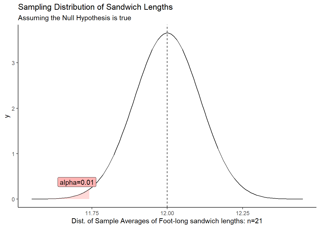
The red area, $\alpha$, shows the probability of getting a sample mean in that tail when the null hypothesis is true. There’s always a chance we get such an extreme value and end up rejecting the null when it is true.

The most common choice for $\alpha$ is $\alpha =0.05$, but other choices include $\alpha =0.1$ and $\alpha =0.01$.

We can set $\alpha$ arbitrarily low to avoid Type I errors, but there’s a cost. The more difficult it is to reject the Null Hypothesis, the more likely we will be to make a Type II Error.

Type II Error: Failing to Reject a FALSE null hypothesis.

If the $\alpha$ value (the probability of committing a Type I error) is very small, the probability of committing a Type II error will be large. Conversely, if $\alpha$ is allowed to be very large, then the probability of committing a Type II error will be very small.

A level of significance of $\alpha =0.05$ seems to strike a good balance between the probabilities of committing a Type I versus a Type II error. However, there may be instances where it will be important to choose a different value for $\alpha$. The important thing is to choose $\alpha$ before you collect your data. Typical choices of $\alpha$ are $0.05$ (most common), $0.1$, and $0.01$.

Visualizing Error

The below graph illustrates the relationship between Type I and Type II errors. The red distribution represents the Null Hypothesis, the sampling distribution of sample mean-lengths of foot-long sandwiches, assuming ${\mu }_0=12$.

The blue distribution represents the “TRUE” distribution with a mean, ${\mu }_{truth}=11.2$. We never know this in the real world, but to illustrate, here is a situation where the true population mean is, in fact, less than 12.

If we set $\alpha =0.01$ (red shaded area), we can see that any sample mean to the right of the cutoff would fail to reject the null hypothesis. This mistake would be a Type II error.

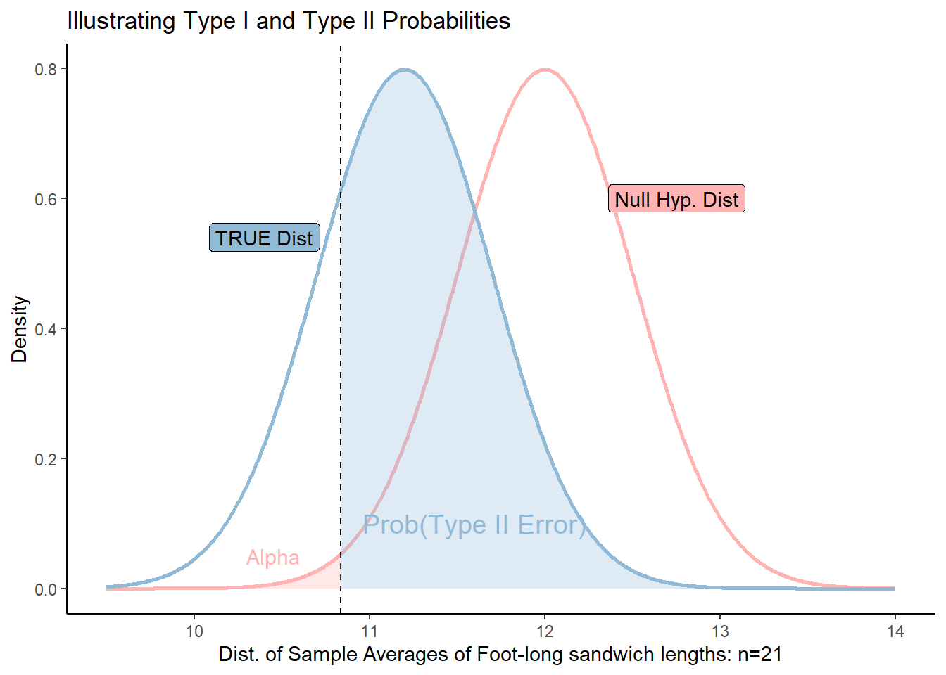
While we don’t know what the “TRUE” distribution is, we can see the relationship between moving the cutoff based on $\alpha$ would do to the probability of failing to reject the null hypothesis even when it is FALSE.