Chi-square Test of Independence

Comparing Categorical Data with Multiple Categories

To test the relationship between 2 categorical variables, we perform a \(\chi^2\) test of independence. [NOTE: The Greek letter, \(\chi\), is pronounced like “ki” in “kite”, not like “chi” in “tai chi”].

We begin a Chi-square test with a contingency table. Recall that a contingency shows the frequency of each combination of categorical variables in a sample.

The Chi-square test statistics is derived by looking at how far away are the observed frequencies away from what we would expect, if there was no relationship between the 2 variables.

Example

Consider the relationship between regular exercise and whether they have a healthy weight. A survey of 200 people showed:

	Healthy Weight	Not Healthy Weight	Row Total
Exercises Regularly	60	20	80
Doesn’t Exercise	40	80	120
Column Total	100	100	200

Does exercising make you more likely to have a healthy weight? Or are the two things completely unrelated?

Expected Counts

Expected counts represent what we would expect to see in each cell of the table if there was no relationship between exercise and weight.

If there’s no relationship, then the proportion of people with a healthy weight should be the same regardless of whether they exercise or not. Similarly, the proportion of people who exercise should be the same regardless of whether they have a healthy weight or not.

Consider the expected number of people who Exercises Regularly and have a Healthy Weight.

Out of the 200 people, 100 have a healthy weight. So, the overall proportion of people with a healthy weight is 100/200 = 0.5 (or 50%). If exercise has no effect on weight, we would expect 50% of the people who exercise to have a healthy weight.

Because a total of 80 people exercise regularly, we would expect \(0.5 * 80 = 40\) people to both exercise regularly and have a healthy weight.

R will calculate the expected counts for every cell automatically.

Comparing Observed and Expected Counts:

To test the hypothesis that there is no relationship between exercise and weight, we compare what we actually observed to what we would expect if there was no relationship. Big differences between the observed and expected counts suggest that there is a relationship between the variables.

• For example, we observed 60 people who exercise and have a healthy weight, but we expected only 40. This is a difference of 20.
• Similarly, we observed 20 people who exercise and don’t have a healthy weight, but we expected 40. This is a difference of -20.

The Chi-Square Test

The chi-square test uses these differences between observed and expected counts to calculate a test statistic. The larger the differences, the larger the test statistic, and the stronger the evidence against the null hypothesis.

Hypothesis Test

The null and alternative hypotheses test for \(\chi^2\) test for independence are always the same.

\[H_0: \text{The row variable is independent of the column variable}\] \[H_A: \text{The row variable is not independent of the column variable}\] While not a fan of the double negative, it serves a technical purpose. Mathematically, we get the same test statistic and p-value if we swap rows and columns. We cannot say the row variable depends on the column variable without also saying that the column variable depends on the row variable.

Think of Alice at the Mad Hatter’s tea party:

“Then you should say what you mean,” the March Hare went on. “I do,” Alice hastily replied; “at least-at least I mean what I say-that’s the same thing, you know.”

“Not the same thing a bit!” said the Hatter. “Why, you might just as well say that ‘I see what I eat’ is the same thing as ‘I eat what I see’!”

“You might just as well say,” added the March Hare, “that ‘I like what I get’ is the same thing as ‘I get what I like’!”

“You might just as well say,” added the Dormouse, which seemed to be talking in its sleep, “that ‘I breathe when I sleep’ is the same thing as ‘I sleep when I breathe’!”

“It is the same thing with you.” said the Hatter,”

So we are resigned to conclude that we have sufficient/insufficient evidence that they are not independent.

Test Statistic

The \(\chi^2\) test statistic measures how far away the observed counts are away from what is expected if the null hypothesis is true.

As with other test statistics, \(\chi^2\) has a probability distribution. We use the probability distribution to calculate a P-value, which measures how likely it is to observe what we observed if the null hypothesis is true.

The \(\chi^2\) test statistic is based on squared differences between observed and expected counts, so it is always positive and right skewed like the F-statistic.

Degrees of Freedom

The shape of the \(\chi^2\) distribution depends on the number of row and column levels. The degrees of freedom determine the shape of the Chi-square probability distribution.

The \(\chi^2\) degrees of freedom are:

\[df = (r-1)(c-1)\] Where \(r\) is the number of rows and \(c\) is the number of columns in a summary table.

Test Requirements

For a Chi-square test to be valid, we need to have enough data so that each of the table cell combinations have adequate representation. This is similar to the 2-sample tests for proportions where we needed at least 10 expected successes and at least 10 expected failures (\(np \ge 10\) and \(n(1-p)\ge10\)), only now we need to check all the combinations.

If all the expected counts are greater than or equal to 5, we can trust the P-value.

Tests for Independence in R

The R code for \(\chi^2\) tests for independence is simple, especially when we have raw data. We can easily create a contingency table using the table_name <- table(col1, col2) function, then insert table_name into the chisq.test(table_name) function.

library(tidyverse)
library(mosaic)
library(rio)
library(ggplot2)

chiropractic <- import('https://raw.githubusercontent.com/byuistats/Math221D_Cannon/master/Data/chiropractic_data.csv')

head(chiropractic,15)

   location motivation
1    Europe   Wellness
2    Europe   Wellness
3    Europe   Wellness
4    Europe   Wellness
5    Europe   Wellness
6    Europe   Wellness
7    Europe   Wellness
8    Europe   Wellness
9    Europe   Wellness
10   Europe   Wellness
11   Europe   Wellness
12   Europe   Wellness
13   Europe   Wellness
14   Europe   Wellness
15   Europe   Wellness

unique(chiropractic$location)

[1] "Europe"        "Australia"     "United States"

unique(chiropractic$motivation)

[1] "Wellness"   "Prevention" "At Risk"    "Sick Role"  "Self Care" 

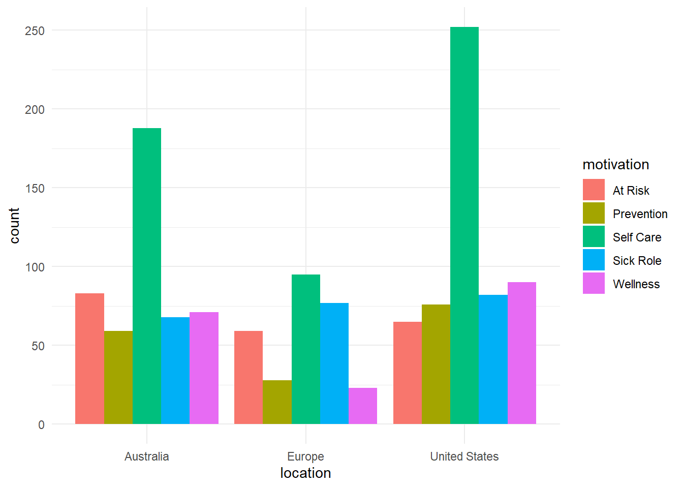
In this dataset, we have a column with “location” indicating the region of the respondents, and the motivation for visiting a chiropractor. Our null and alternative hypotheses are:

\[H_0: \text{Why you go to a chirpractor is independent of where you live}\] \[H_0: \text{Why you go to a chirpractor is not independent of where you live}\]

chiro_table <- table(chiropractic$location, chiropractic$motivation)
chiro_table

               
                At Risk Prevention Self Care Sick Role Wellness
  Australia          83         59       188        68       71
  Europe             59         28        95        77       23
  United States      65         76       252        82       90

chisq.test(chiro_table)

    Pearson's Chi-squared test

data:  chiro_table
X-squared = 49.743, df = 8, p-value = 4.58e-08

Conclusion: We have sufficient evidence to conclude that why you go to the chiropractor is not independent of where you live.

Check the Requirements

Check that all the expected counts are greater than 5. We can extract the expected counts from the chisq.test() using the $expected and see if they are all greater than 5.

chisq.test(chiro_table)$expected

               
                 At Risk Prevention Self Care Sick Role Wellness
  Australia     73.77128   58.09043  190.6649  80.89894 65.57447
  Europe        44.35714   34.92857  114.6429  48.64286 39.42857
  United States 88.87158   69.98100  229.6922  97.45821 78.99696

A useful trick is to use a logical operator to test if each value is greater than 5:

chisq.test(chiro_table)$expected >= 5

               
                At Risk Prevention Self Care Sick Role Wellness
  Australia        TRUE       TRUE      TRUE      TRUE     TRUE
  Europe           TRUE       TRUE      TRUE      TRUE     TRUE
  United States    TRUE       TRUE      TRUE      TRUE     TRUE

If they are all TRUE, then your requirements are satisfied.

Visualization

We can use ggplot() to create nice bar charts to help interpret the results.

ggplot(chiropractic, aes(x = location, fill = motivation)) +
  geom_bar(position = "dodge") +
  theme_minimal()

Summarized Data

Sometimes we get data that are already summarized instead of raw data in columns. This often comes with a column that is actually a category label.

Suppose we have a summary table:

Gender	Republican	Democrat	Independent
Female	250	300	50
Male	200	150	50

This contains a column for Gender, which is not part of the summary table that is required to input into the chisq.test() function.

We can use the select() statement to include only the columns with summary data.

politics_table <- politics %>% 
  select(Republican, Democrat, Independent)

We can now use politics_table in the chisq.test() function.

Your Turn

A public opinion poll surveyed a simple random sample of 1000 voters. Respondents were classified by gender (female or male) and by voting preference (Republican, Democrat, or Independent). The results are presented here:

voting <- data.frame(c("Female", "Male"), 
           c(250, 200),
           c(300, 150),
           c(50,50))
names(voting) <- c("Gender", "Republican", "Democrat", "Independent")

knitr::kable(voting)

Gender	Republican	Democrat	Independent
Female	250	300	50
Male	200	150	50

Do men’s voting preferences differ significantly from women’s voting preferences?

Use a level of significance of \(\alpha = 0.05\)

QUESTION: State the null and alternative hypothesis:

Ho:
Ha:

Use the voting data table created above to make a new table that does not include the Gender column. ( NOTE: You may have to run the code chunk above.)

clean_voting <- voting %>%
  select()

QUESTION: Perform a hypothesis test:

QUESTION: What is the test statistic for this test?
ANSWER:

QUESTION: How many degrees of freedom are there for this test?
ANSWER:

QUESTION: What is the p-value?
ANSWER:

QUESTION: What is your conclusion?
ANSWER: