Statistical Significance

Introduction

Statistical significance is a crucial concept for determining whether the results observed in a study are likely due to a real effect or simply due to chance. It’s a core component of hypothesis testing.

Reviw: P-value

The \(P\)-value is the probability of observing results as extreme as or more extreme than the results obtained in your sample assuming the null hypothesis is true. In other words, it indicates how likely it is to see the data you did if there was actually no effect present.

A small p-value suggests strong evidence against the null hypothesis, while a large p-value suggests the observed data are consistent with sample-to-sample variability.

Significance Level: Alpha (\(\alpha\))

Before starting a study, we set a threshold that can be used to determine if the \(P\)-value is small enough to reject the null hypothesis. This number is called the level of significance and is denoted by the symbol \(\alpha\) (pronounced “alpha”.)

Common values for \(\alpha\) are 0.05, 0.01 and 0.1.

We will use the same decision rule for all hypothesis tests:

1. If the \(P\)-value is less than \(\alpha\), we reject the null hypothesis.
   
2. If the \(P\)-value is greater than \(\alpha\), we fail to reject the null hypothesis.

Memory Aid: If \(P\) is low, reject \(H_O\)

Where “low” means less than \(\alpha\).

Mistaking Randomness for Signal

We can never be 100% certain that the signal observed in our sample was not just noise. Randomization is used to design statistical experiments to avoid bias in our samples, but sometimes that randomness can lead to results that look significant just by chance.

Consider a clinical trial looking at 5-year survival rates for a new cancer therapy with 3 different levels of the treatment. We randomly assign patients to each treatment group.

There is a chance that the hardiest patients all end up in the same treatment group making it look like that treatment is better, but it wasn’t because of the treatment.

When we conclude that there is a relationship between X and Y, when what we observed was actually “noise”, we have committed a Type I error.

DEFINITION: Type I Error: Rejecting a TRUE null hypothesis. In some contexts this is called a FALSE POSITIVE

Because \(\alpha\) is our decision point for rejecting the null hypothesis, \(\alpha\) is the probability of rejecting a TRUE null hypothesis, meaning \(\alpha\) is the probability of a Type I error.

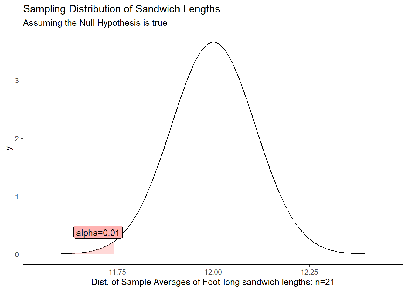
Let’s see what an \(\alpha = 0.01\) looks like in the case of against the foot-long sandwiches:

The red area, \(\alpha\), shows the probability of getting a sample mean in that tail when the null hypothesis is true. There’s always a chance we get such an extreme value and end up rejecting the null when it is true.

If we make \(\alpha\) too small, we will reject \(H_0\) less often, thereby avoiding Type I errors. But that means that we are MORE likely to fail to reject the null hypothesis when we SHOULD have rejected it. This is a Type II error.

DEFINITION: Type II Error: Failing to Reject a FALSE null hypothesis. In some contexts this is called a FALSE NEGATIVE

For example, if we failed to find evidence that the new cancer therapy worked but it really WAS effective, then we missed out on an a new, life-saving breakthrough.

Choosing Alpha and Understanding Error Types

Choosing an appropriate alpha level involves balancing the risk of making Type I and Type II errors

The “best” choice for alpha depends on the context of the research. In exploratory research, a higher alpha (e.g., 0.10) might be acceptable to avoid missing potentially important effects. In situations where making a false positive conclusion could have serious consequences, a lower alpha (e.g., 0.01 or even lower) is preferred.

If the \(\alpha\) value (the probability of committing a Type I error) is very small, the probability of committing a Type II error will be large. Conversely, if \(\alpha\) is allowed to be very large, then the probability of committing a Type II error will be very small.

A level of significance of \(\alpha=0.05\) seems to strike a good balance between the probabilities of committing a Type I versus a Type II error. However, there may be instances where it will be important to choose a different value for \(\alpha\). The important thing is to choose \(\alpha\) before you collect your data. Typical choices of \(\alpha\) are \(0.05\) (most common), \(0.1\), and \(0.01\).

Visualizing Error

The graph below illustrates the relationship between Type I and Type II errors. The red distribution represents the Null Hypothesis, the sampling distribution of mean lengths of foot-long sandwiches, assuming \(\mu_0=12\).

The blue distribution represents the “TRUE” distribution with a mean, \(\mu_{truth}=11.2\). We never know this in the real world, but to illustrate, here is a situation where the true population mean is, in fact, less than 12. The right decision would be to REJECT \(H_0\).

If we set \(\alpha = 0.01\) (red shaded area), we can see that any sample mean to the right of the cutoff would fail to reject the null hypothesis. This mistake would be a Type II error.

While we don’t know what the “TRUE” distribution is, we can see the relationship between moving the cutoff based on \(\alpha\) would do to the probability of failing to reject the null hypothesis even when it is FALSE.