Probability
Introduction to Probability and Distributions
Probability plays a fundamental role in Statistics. In this section, we introduce the basic rules of probability for discrete events and introduce the idea of a probability distribution for continuous events. We provide a few examples of continuous probability distributions that will be used for making inference about a population.
The Concept of Probability
Probability measures the likelihood of an event occurring. It is a quantifiable measure between 0 (impossible) to 1 (certain).
We can calculate probabilities for discrete and continuous events and will discuss each below.
Discrete Events
A discrete event refers to an event that has a distinct, countable outcome. For example:
- Flipping a coin has 2 possible outcomes: Heads or Tails
- Rolling a die has 6 possible outcomes: 1-6
- The number of red-headed students in a classroom
The key characteristic is that we can count up the number of times a given event occurs. For example, you can roll a dice 100 times and count how many 1’s, 2’s, 3’s, etc. you get.
We call each possible outcome an “event” and write the probability of an event: \(P(E)\). We can estimate the probability of an event by trying experiments over time, such as rolling a die over and over, counting up the number of occurrences of events and dividing by the number of rolls.
Fundamental Rules for Discrete Events
Rule 1: The Probability of an Event
\[ 0 \leq P(E) \leq 1 \]
- Certain Event
\[ P(\text{certain}) = 1 \]
- Impossible Event
\[ P(\text{impossible}) = 0 \]
Rule 2: Complement Rule
\[ P(\text{not } E) = 1 - P(E) \]
Rule 3: Total Probability
\[ \sum_{i=1}^n P(E_i) = 1 \]
Practice
Use the probabilty rules above to answer the following questions.
QUESTION: In a political poll, 40% of respondents favor candidate A, 35% favor candidate B, and the rest are undecided. If one respondent is selected at random, what is the probability that they either favor candidate A or are undecided?
ANSWER:
QUESTION: In a survey of 288 BYU-I students, 144 said they prefer Redneck Mixers from Great Scott’s for their soda, 58 said they prefer Swig and 68 preferred Fixxology. The rest are heathens with questionable orthodoxy who have a distaste for non-alcoholic sparkling drinks. What is the probability of randomly selecting a student that hates delicious beverages?
ANSWER:
Continuous Probability Distributions
In many situations, we can’t count the number of specific events. This typically occurs when we are collecting quantitative data such as heights. In practice, we do not have an infinite resolution for measuring heights. We might measure to the quarter inch, or the centimeter. While rounding makes things a little more like a discrete event, we understand that height is a continuous measurement and typically model it with a continuous probability distribution.
Continuous probability distributions describe how probabilities are spread over all possible outcomes. Because there are technically an infinite number of possible outcomes on a continuous scale, the probability of any specific event is zero. Weird, right?
In continuous cases, it doesn’t make sense to calculate the probability of exactly an event, \(E\). It makes more sense to think of probabilities in relation to specified values. For example, what’s the probability that a person is shorter then 72.1254 inches. Or what’s the probability of randomly selecting a person who makes MORE than $182,000 a year.
The Calculus is required to calculate probabilities for continuous probability distributions. Fortunately, you do NOT need to know any calculus for this class because computers will perform all the calculations for us. However, it is important to understand a few basic principles for continuous probability distributions.
The Normal Distribution
We will use the Normal Distribution to illustrate the probability rules for continuous probability distributions. The rules apply to any continuous probability distribution, but the normal distribution is one of the fundamental probability distributions in statistics. We will learn more about it in future lessons. For now, we use it only to illustrate the probability rules for continuous distributions.
The normal distribution is like a smooth histogram that is perfectly symmetric around the mean and has a standard deviation that determines how spread out the distribution is. Consider below a histogram of Major League Baseball batting averages:
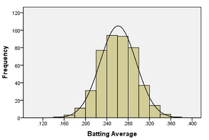 The smooth line is a normal distribution superimposed onto the histogram of the data. Using our data, we can calculate percentiles by adding up
Suppose we want to estimate the probability that a randomly selected player will have a batting average that is greater than 0.280. One way to do this would be to find the proportion of players in the data set who have a batting average above 0.280. We can do this by finding the number of players who fall into each of the red-colored bins below and dividing this number by the total number of players.
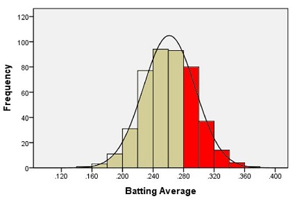 In other words, we could find the proportion of the total area of the bars that is shaded red out of the combined area of all the bars. This gives us the proportion of players whose batting averages are greater than 0.280.
Out of the 446 players listed, there are a total of 133 players with batting averages over 0.280. This suggests that the proportion of players whose batting average exceeds 0.280 is:
\[\displaystyle{\frac{133}{446}} = 0.298\]
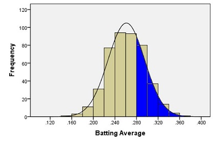
Alternatively, we can use the fact that the data follow a bell-shaped distribution to find the probability that a player has a batting average above 0.280.
Probability Rules for Continuous Distributions
The principles are roughly the same as for discrete events.
- 1. Total Probability:
\[\text{The Total} \textbf{ area under the curve} \text{ is equal to 1.}\]
- 2. P(E < a)
The probability that an event is less than some value, \(a\), is the area under the curve to the left of \(a\).

- 3. P(E > b)
The probability that an event is greater than some value, \(b\), is the area under the curve to the right of \(b\).

- 4. P(a < E < b)
The probability of being between 2 numbers is the area under the curve between the 2 numbers:

4. The Complement Rule
The probability that a continuous random variable does not fall within an interval ([a, b]) is:
\[ P(\text{not in } [a, b]) = 1 - P(a \leq X \leq b) \]

Key Probability Distributions
Below are several examples of continuous probability distributions that will be used in this class for making inference about populations in different situations.
Most of the distributions below change shape depending on certain attributes of our sample. However, they all share 2 important characteristics:
- The total area under the curve is 1 (total probability)
- We can use R to calculate the probabilities of certain events for all of these distributions.
NOTE: Right now, it’s only important to be aware that there are different probability distributions.
| Distribution | Examples | Shape Characteristics | Key Parameters |
|---|---|---|---|
| Z: Standard Normal |  |
Bell-shaped, symmetric | (mean=0, std. dev. = 1) |
| Student’s t |  |
Bell-shaped, heavier tails | (df) |
| F-Distribution |  |
Right skewed, always positive | (df_1, df_2) |
| Chi-Squared |  |
Right-skewed, always positive | (df) |