One-Sample T-test

One-Sample T-test and Confidence Intervals

Lesson Objectives

By the end of this lesson, you should be able to:

Recognize when a one mean inferential procedure is appropriate
Perform a hypothesis test for one mean using the following steps:
1. State the null and alternative hypotheses
2. Calculate the test-statistic, degrees of freedom and P-value using R
3. Assess statistical significance in order to state the conclusion for the hypothesis test in context of the research question
4. Check the requirements for the hypothesis test
Create a confidence interval for one mean using the following steps:
1. Calculate a confidence interval for a given level of confidence using R
2. Interpret the confidence interval
3. Check the requirements of the confidence interval
State the properties of the Student’s t-distribution

Review

Statistical Inference

Statistical Inference is the practice of using data sampled from a population to make conclusions about population parameters.

The two primary methods of statistical inference are:

Confidence Intervals
Hypothesis Testing

Recall that when we know what the population standard deviation, $\sigma$, for individuals, and are confident that the distribution of sample means is approximately normal, we can use a $z$-score for a mean and the Standard Normal Distribution to calculate probabilities.

\[ z= \frac{\bar{x} - \mu}{\frac{\sigma}{\sqrt{n}}}\]

We can use pnorm(z) to get the left-tail probability of observing our sample mean for a given (or hypothesized) $\mu$.

Though rare, there are situations where we might know the population standard deviation from published research or census data. For example, standardized test organizations publish population-level summaries which would allow us to test how our sample compares to the general population using the Z formula.

Student’s T-Distribution

In most cases, we perform statistical analyses on samples from a population where we don’t know the population standard deviation, $\sigma$.

A simple solution is to use the sample standard deviation, $s$, instead of $\sigma$.

The test statistic for a 1-sample t-test looks a lot like a z-score, but substitutes $\sigma$ with the sample standard deviation, $s$.

\[ t = \frac{\bar{x} - \mu}{\frac{s}{\sqrt{n}}}\]

As with the normal distribution above, we can use R to calculate probabilities with the $t$-distribution. For a given sample size, $n$, and the calculated $t$-value above, we can use the function pt(t_value, df=n-1) to get the probability of getting a sample mean less than our observed $\bar{x}$.

RECALL: Degrees of Freedom for a $t$-distribution are defined:

\[df = n-1 \]

Calculating P-values by hand with the T-distribution (One out of ten. Would NOT RECOMMENDED)

Here is an example of performing a hypothesis test using the $t$-distribution by hand.

Suppose we have a sample of 25 test scores of Math 221 students. We believe that the true population mean of Math 221 students is significantly higher than overall average of 50.

Our null and alternative hypothesis are as follows:

\[ H_0: \mu_{\text{M221 Students}} = 50 \] We would read this: The population average test score of Math 221 students is equal to the general population average of 50.

\[ H_a: \mu_{\text{M221 Students}} > 50 \] We would read this: The population average test score of Math 221 students is greater than the general population average of 50.

NOTE: The direction of the alternative hypothesis (“greater”, “less”, “two.sided”) will depend on the context of the research question. If you believe your drug lowers cholesterol, then you may have alternative = "less". If you genuinely do not know if the population mean is higher or lower, you can use alternative = "two.sided".

We could then use favstats(data) to get everything we need to plug into the formula and calculate the probabilities using the $t$-distribution.

library(mosaic)

# we can use the t-distribution, pt(), just like pnorm() but must also add the degrees of freedom

test_scores <- c(88,81,27,92,46,79,67,44,46,88,21,60,71,81,79,52,100,44,42,58,52,48,83,65,98)

# Save the output of the favstats() function  

summary_stats <- favstats(test_scores)
summary_stats

 min Q1 median Q3 max  mean       sd  n missing
  21 46     65 81 100 64.48 21.96232 25       0

# Use the output to extract the important values for calculating t:  
xbar <- summary_stats$mean
s <- summary_stats$sd
n <- summary_stats$n

# Calculate the standard deviation of a sample mean:  
s_xbar = s / sqrt(n)

# Hypothesized Mean:
mu_0 <- 50


t <- (xbar - mu_0) / s_xbar
t

[1] 3.296556

# Probability of getting a test statistic at least as extreme as the one we observed if the null hypothesis is true
p_value <- 1-pt(t, df = n-1)
p_value

[1] 0.00151866

Question: What is the test statistic, $t$?
Answer:

Question: What is the probability of observing $t$ “greater” then the one we observed if the population mean was really 50? (The P-value)
Answer:

The Easy Way

The good news is that we can use R functions with the data directly and get all the calculations automatically.

Let’s redo the example above using the t.test() function in R.

Using the t.test() function for a hypothesis test requires inputting the data, the hypothesized mean, $\mu$, and the direction of the alternative hypothesis.

NOTE: The default parameters for the t.test() function are: t.test(data, mu = 0, alternative = "two.sided").

# One-sided Hypothesis Test
t.test(test_scores, mu = 50, alternative = "greater")


    One Sample t-test

data:  test_scores
t = 3.2966, df = 24, p-value = 0.001519
alternative hypothesis: true mean is greater than 50
95 percent confidence interval:
 56.96501      Inf
sample estimates:
mean of x 
    64.48

Dig through the output and answer the following questions:

Question: What is the test statistic, $t$?
Answer:

Question: What is the P-value?
Answer:

Check that your answers match the “by hand” method above.

QUESTION: What is your conclusion based on $\alpha=0.05$?
ANSWER: Because P-value < 0.05 we reject the null hypothesis in favor of the alternative.

Question: State your conclusion in context of our research question?
Answer: We have sufficient evidence to conclude that Math 221 students are more extroverted than the general population, on average.

Confidence Interval Review

We can also use the t.test() function to create confidence intervals. Confidence intervals are always 2-tailed and are typically written in the form: (lower limit, upper limit).

Confidence intervals do not assumed anything about $\mu$, so an efficient way to get a confidence interval for a given set of data is to leave out anything relating to the hypotheses and extract only the confidence interval.

Recall that to extract only the confidence interval output, we can use $.

t.test(test_scores, conf.level = .99)$conf.int

[1] 52.19455 76.76545
attr(,"conf.level")
[1] 0.99

Question: Describe in words the interpretation of the confidence interval in context of Extroversion.
Answer: I am 99% confident that the true population mean test score for Math 221 students is between 52.19455 and 76.76545.

Checking Requirements

These confidence intervals and hypothesis tests depend on the assumption that the distribution of sample means is normally distributed.

Recall that the distribution of sample means is approximately normal if:

The underlying population is normally distributed
We have a sufficiently large sample size ($n>30$)

For the above Extroversion data, we have $n=404$ which is much larger than 30.

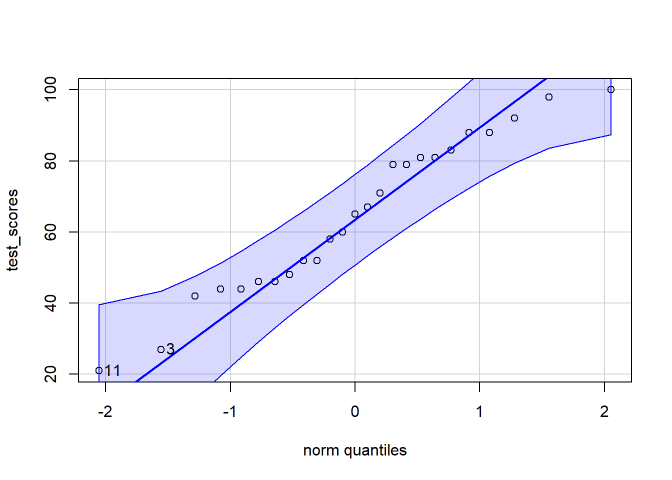
If my sample size was small, I could check the qqPlot(), which I demonstrate here:

library(car)

qqPlot(test_scores)

[1] 11  3

Your Turn

Body Temperature Data

The dataset below contains information about body temperatures of healthy adults.

Load the data:

# These lines load the data into the data frame body_temp:

body_temp <- import("https://byuistats.github.io/M221R/Data/body_temp.xlsx")

Error in import("https://byuistats.github.io/M221R/Data/body_temp.xlsx"): could not find function "import"

Review the Data

Create a table of summary statistics for temperature:

Visualize the Data

Create a histogram to visualize the body temperature data.

Question: Describe the general shape of the distribution.
Answer:

Analyze the Data

It’s widely accepted that normal body temperature for healthy adults is 98.6 degrees Fahrenheit.

Suppose we suspect that the average temperature is different than 98.6

Use a significance level of $\alpha = 0.01$ to test whether the mean body temperature of healthy adults is equal to 98.6 degrees Fahrenheit.

Question: What is the P-value?
Answer:

QUESTION: What is your conclusion?
ANSWER:

Confidence Interval

Create a 99% confidence interval for the true population average temperature of healthy adults.

Check the requirements for the t-test ($n>30$ or qqPlot()):

QUESTION: Are the requirements for the t-test satisfied?
ANSWER: