CBE <- read.table("data/cbe.dat", header = T)
Elec.ts <- ts(CBE[, 3], start = 1958, freq = 12)
layout(c(1, 1, 2, 3))
plot(Elec.ts)
plot(diff(Elec.ts))
plot(diff(log(Elec.ts)))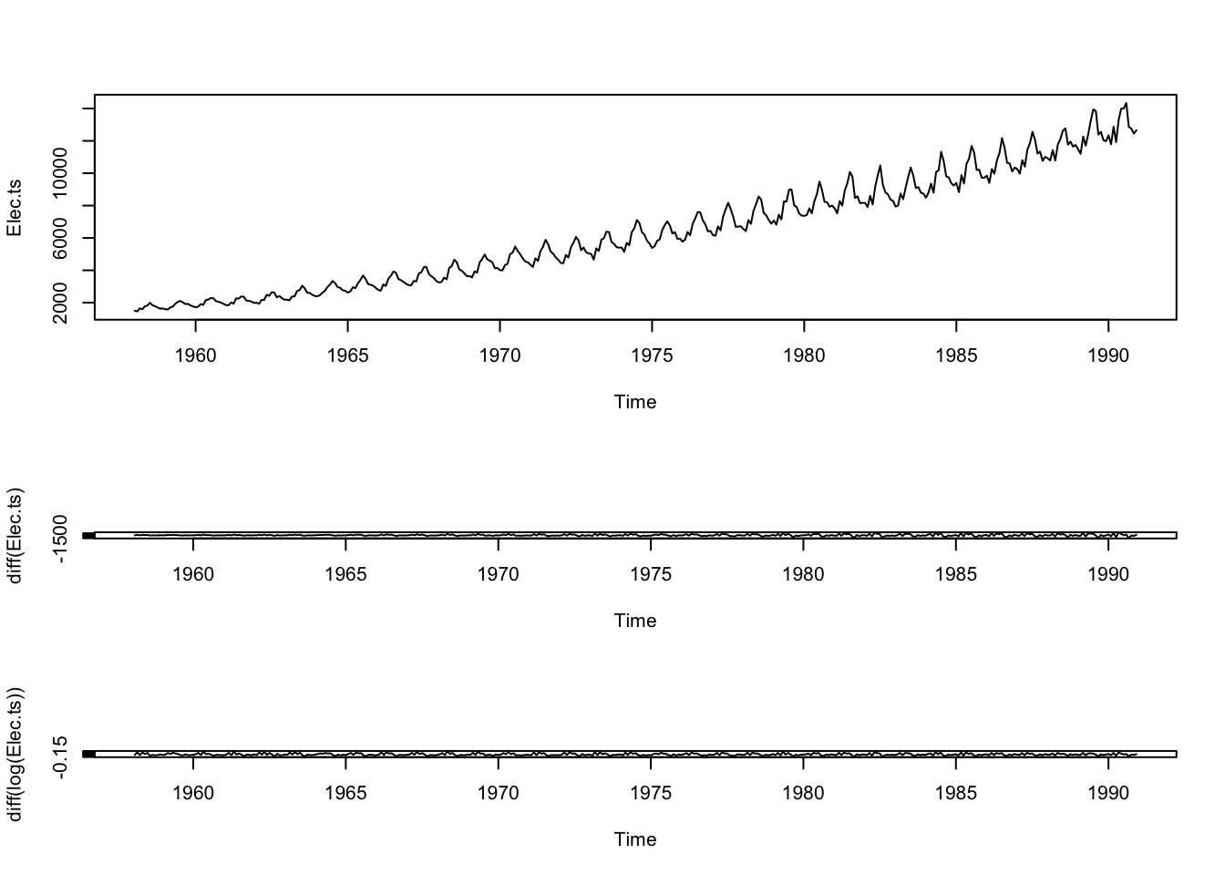
In this chapter, we extend the random walk model to include autoregressive and moving average terms. As the differenced series needs to be ‘integrated’ to recover the original series, the underlying stochastic process is called autoregressive integrated moving average, abbreviated to ARIMA.
We would like to note that the use of the R package tseries for GARCH models appears to be inferior with the addition of the rugarch package (see paper). Currently, no tidyverse developed package supports GARCH.
A short introduction to the rugarch package is helpful to discover more uses of the package.
Book code
CBE <- read.table("data/cbe.dat", header = T)
Elec.ts <- ts(CBE[, 3], start = 1958, freq = 12)
layout(c(1, 1, 2, 3))
plot(Elec.ts)
plot(diff(Elec.ts))
plot(diff(log(Elec.ts)))
Tidyverts code
pacman::p_load("tsibble", "fable", "feasts",
    "tsibbledata", "fable.prophet",
    "tidyverse", "patchwork")
cbe <- read_table("data/cbe.dat")

elec_ts <- cbe |>
  select(elec) |>
  mutate(
    date = seq(
      ymd("1958-01-01"),
      by = "1 months",
      length.out = n()),
      year_month = tsibble::yearmonth(date)) |>
  as_tsibble(index = year_month)

elec_ts |>
  mutate(
    `Diff series` = elec - lag(elec),
    `Diff log-series` = log(elec) - lag(log(elec))) |>
  pivot_longer(
    cols = all_of(c("elec", "Diff series", "Diff log-series"))) |>
  mutate(name = factor(name, levels =c("elec","Diff series", "Diff log-series"))) |>
  ggplot(aes(x = date, y = value)) +
  geom_line() +
  facet_wrap(~name, ncol = 1, scales = "free", strip.position = "left") +
  labs(x = "Time", y = "") +
  scale_x_date(breaks = "5 years", date_labels = "%Y") +
  theme_bw()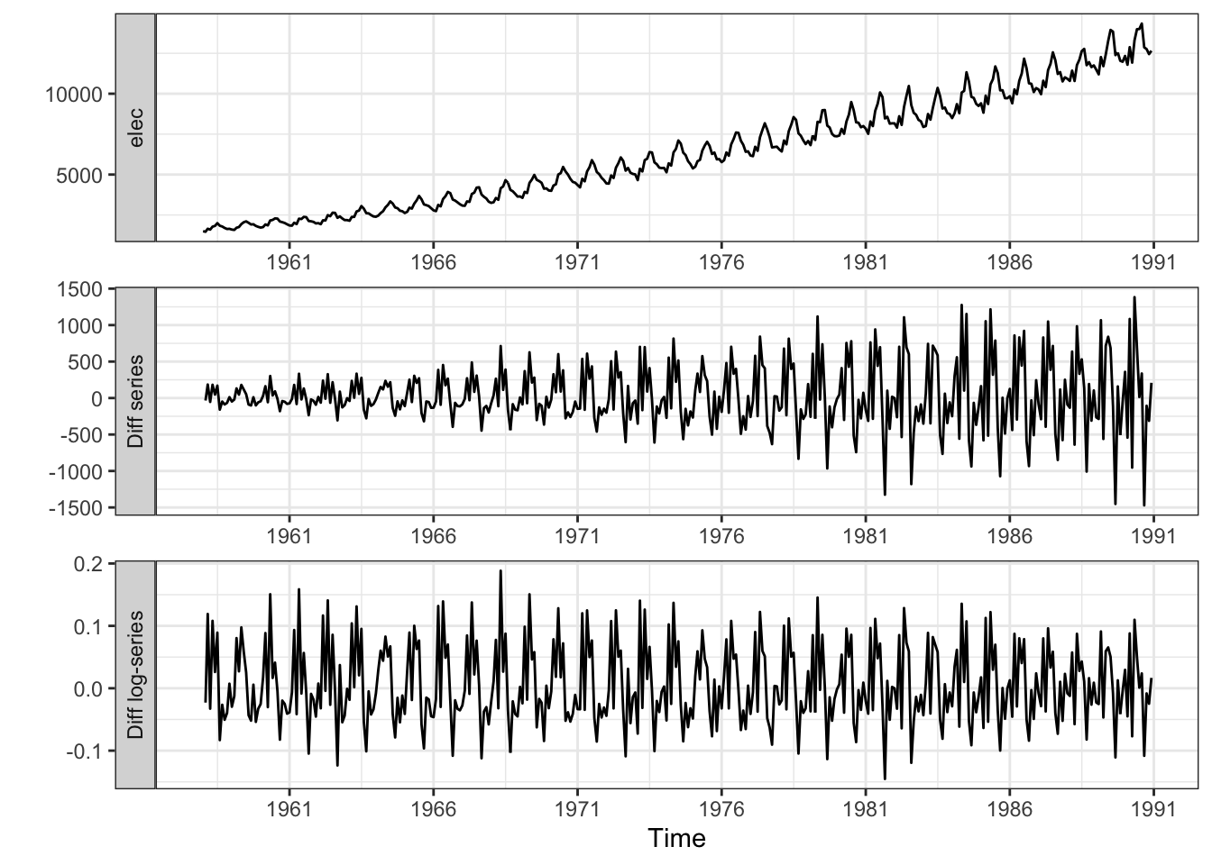
pacman::p_load("tsibble", "fable", "feasts",
    "tsibbledata", "fable.prophet",
    "tidyverse", "patchwork")
cbe <- read_table("data/cbe.dat")
elec_ts <- cbe |>
  select(elec) |>
  mutate(
    date = seq(
      ymd("1958-01-01"),
      by = "1 months",
      length.out = n()),
      year_month = tsibble::yearmonth(date)) |>
  as_tsibble(index = year_month)

elec_ts |>
  mutate(
    `Diff series` = elec - lag(elec),
    `Diff log-series` = log(elec) - lag(log(elec))) |>
  pivot_longer(
    cols = all_of(c("elec", "Diff series", "Diff log-series"))) |>
  mutate(name = factor(name, levels =c("elec","Diff series", "Diff log-series"))) |>
  ggplot(aes(x = date, y = value)) +
  geom_line() +
  facet_wrap(~name, ncol = 1, scales = "free", strip.position = "left") +
  labs(x = "Time", y = "") +
  scale_x_date(breaks = "5 years", date_labels = "%Y") +
theme_bw()Book code
set.seed(1)
x <- w <- rnorm(1000)
for (i in 3:1000) x[i] <- 0.5 * x[i - 1] + x[i - 1] -
  0.5 * x[i - 2] + w[i] + 0.3 * w[i - 1]
arima(x, order = c(1, 1, 1))
Call:
arima(x = x, order = c(1, 1, 1))

Coefficients:
         ar1     ma1
      0.4235  0.3308
s.e.  0.0433  0.0450

sigma^2 estimated as 1.067:  log likelihood = -1450.13,  aic = 2906.26
Tidyverts code
set.seed(1)
x <- w <- rnorm(1000)
for (i in 3:1000) x[i] <- 0.5 * x[i - 1] + x[i - 1] -
  0.5 * x[i - 2] + w[i] + 0.3 * w[i - 1]
tibble(x = x) |>
  mutate(time = 1:n()) |>
  as_tsibble(index = time) |>
  model(arima = ARIMA(x ~ pdq(1, 1, 1) + PDQ(0, 0, 0))) |>
  tidy()
# A tibble: 2 × 6
.model term estimate std.error statistic p.value
<chr> <chr> <dbl> <dbl> <dbl> <dbl>
1 arima ar1 0.423 0.0433 9.79 1.11e-21
2 arima ma1 0.331 0.0450 7.35 4.02e-13x <- arima.sim(model = list(
order = c(1, 1, 1),
ar = 0.5,
ma = 0.3),
n = 1000)
arima(x, order = c(1, 1, 1))
Call:
arima(x = x, order = c(1, 1, 1))

Coefficients:
         ar1     ma1
      0.5567  0.2502
s.e.  0.0372  0.0437

sigma^2 estimated as 1.079: log likelihood = -1457.45, aic = 2920.91tibble(x = arima.sim(model = list(
order = c(1, 1, 1),
ar = 0.5,
ma = 0.3),
n = 1000)) |>
mutate(time = 1:n()) |>
as_tsibble(index = time) |>
model(arima = ARIMA(x ~ pdq(1, 1, 1) + PDQ(0, 0, 0))) |>
tidy()# A tibble: 2 × 6
.model term estimate std.error statistic p.value
<chr> <chr> <dbl> <dbl> <dbl> <dbl>
1 arima ar1 0.475 0.0380 12.5 2.42e-33
2 arima ma1 0.376 0.0395 9.53 1.19e-20set.seed(1)
x <- w <- rnorm(1000)
for (i in 3:1000) x[i] <- 0.5 * x[i - 1] + x[i - 1] -
0.5 * x[i - 2] + w[i] + 0.3 * w[i - 1]
tibble(x = x) |>
mutate(time = 1:n()) |>
as_tsibble(index = time) |>
model(arima = ARIMA(x ~ pdq(1, 1, 1) + PDQ(0, 0, 0))) |>
tidy()
tibble(x = arima.sim(model = list(
    order = c(1, 1, 1),
    ar = 0.5,
    ma = 0.3),
    n = 1000)) |>
  mutate(time = 1:n()) |>
  as_tsibble(index = time) |>
  model(arima = ARIMA(x ~ pdq(1, 1, 1) + PDQ(0, 0, 0))) |>
tidy()Book code
Beer.ts <- ts(CBE[, 2], start = 1958, freq = 12)
Beer.ima <- arima(Beer.ts, order = c(0, 1, 1))
Beer.ima
Call:
arima(x = Beer.ts, order = c(0, 1, 1))

Coefficients:
          ma1
      -0.3334
s.e.   0.0558

sigma^2 estimated as 360.4:  log likelihood = -1723.27,  aic = 3450.53
Tidyverts code
cbe <- read_table("data/cbe.dat")
beer_ts <- cbe |>
  select(beer) |>
  mutate(
    date = seq(
      ymd("1958-01-01"),
      by = "1 months",
      length.out = n()),
      year_month = tsibble::yearmonth(date)) |>
  as_tsibble(index = year_month)

beer_arima <- beer_ts |>
  model(arima = ARIMA(beer ~ pdq(0, 1, 1) + PDQ(0, 0, 0)))

tidy(beer_arima)
# A tibble: 1 × 6
.model term estimate std.error statistic p.value
<chr> <chr> <dbl> <dbl> <dbl> <dbl>
1 arima ma1 -0.333 0.0558 -5.97 0.00000000515acf(resid(Beer.ima))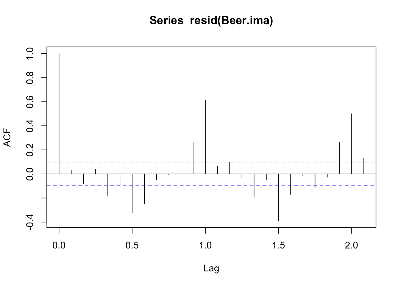
beer_arima |>
  residuals() |>
  ACF() |>
  autoplot()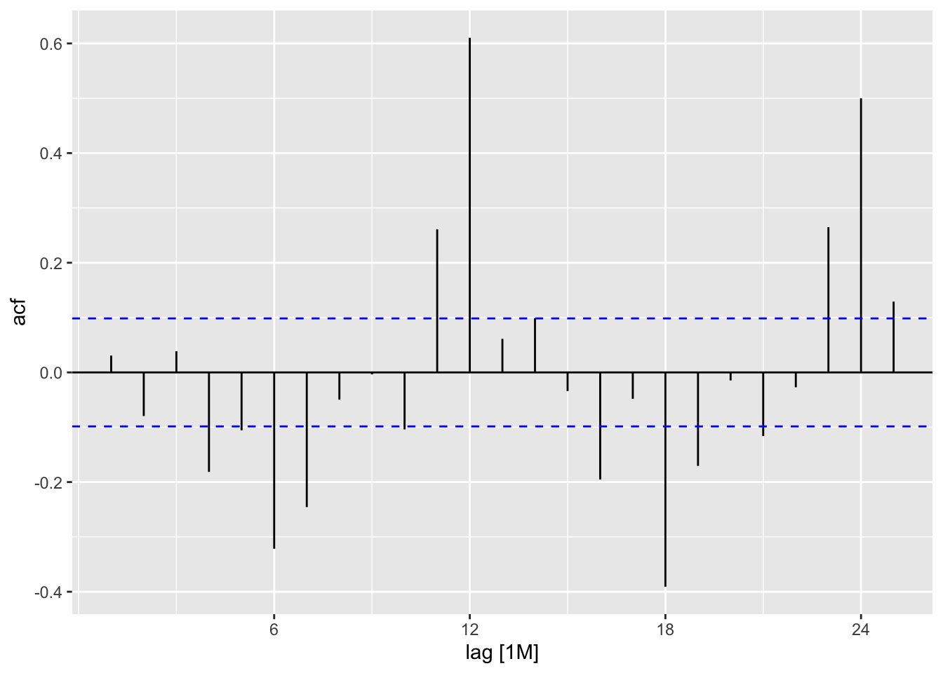
Beer.1991 <- predict(Beer.ima, n.ahead = 12)
sum(Beer.1991$pred)
[1] 2365.412beer_1991 <- beer_arima |>
forecast(h = "12 months")
pull(beer_1991, .mean) |> sum()[1] 2365.412cbe <- read_table("data/cbe.dat")
beer_ts <- cbe |>
select(beer) |>
mutate(
date = seq(
ymd("1958-01-01"),
by = "1 months",
length.out = n()),
year_month = tsibble::yearmonth(date)) |>
as_tsibble(index = year_month)
beer_arima <- beer_ts |>
model(arima = ARIMA(beer ~ pdq(0, 1, 1) + PDQ(0, 0, 0)))
tidy(beer_arima)
beer_arima |>
residuals() |>
ACF() |>
autoplot()
beer_1991 <- beer_arima |>
  forecast(h = "12 months")

pull(beer_1991, .mean) |> sum()Book code
aic1 <- AIC(arima(log(Elec.ts),
  order = c(1,1,0),
  seas = list(order = c(1,0,0), 12)))
aic2 <- AIC(arima(log(Elec.ts),
  order = c(0,1,1),
  seas = list(order = c(0,0,1), 12)))
c("aic1" = aic1, "aic2" = aic2)
aic1 aic2
-1764.741 -1361.586 Tidyverts code
elec_ts |>
  model(
    ar_model = ARIMA(log(elec) ~ 1 +
      pdq(1, 1, 0) +
      PDQ(1, 0, 0)),
    ma_model = ARIMA(log(elec) ~ 1 +
      pdq(0, 1, 1) +
      PDQ(0, 0, 1))) |>
  glance() |>
  pull(AIC)
[1] -1763.076 -1362.217get.best.arima <- function(x.ts, maxord = c(1,1,1,1,1,1)) {
best.aic <- 1e8
n <- length(x.ts)
for (p in 0:maxord[1]) for(d in 0:maxord[2]) for(q in 0:maxord[3])
for (P in 0:maxord[4]) for(D in 0:maxord[5]) for(Q in 0:maxord[6])
{
fit <- arima(x.ts, order = c(p,d,q),
seas = list(order = c(P,D,Q),
frequency(x.ts)), method = "CSS")
fit.aic <- -2 * fit$loglik + (log(n) + 1) * length(fit$coef)
if (fit.aic < best.aic)
{
best.aic <- fit.aic
best.fit <- fit
best.model <- c(p,d,q,P,D,Q)
}
}
list(best.aic, best.fit, best.model)
}
best.arima.elec <- get.best.arima(
log(Elec.ts),
maxord = c(2,2,2,2,2,2))
best.fit.elec <- best.arima.elec[[2]]
acf(resid(best.fit.elec))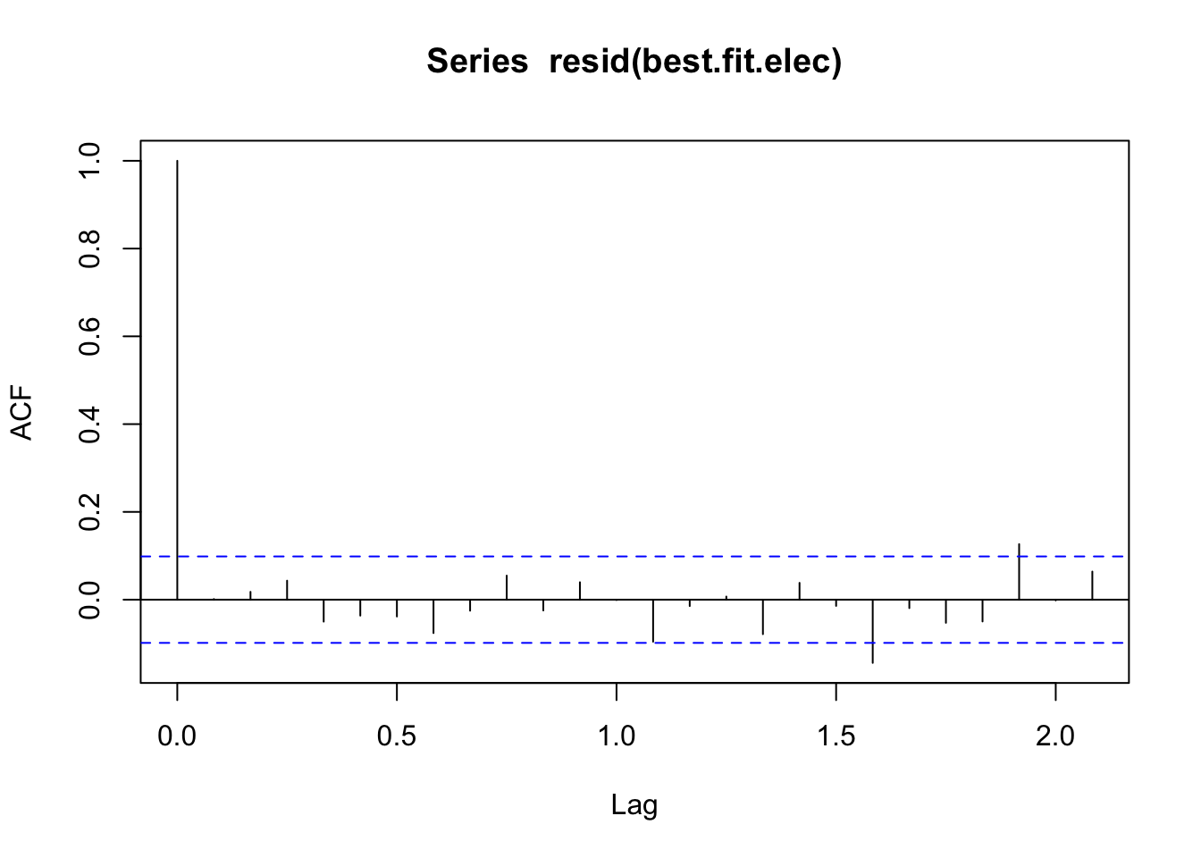
best_fit_elec <- elec_ts |>
  model(
    ar_model = ARIMA(log(elec) ~ 1 +
      pdq(0:2, 0:2, 0:2) +
      PDQ(0:2, 0:2, 0:2), approximation = TRUE))

best_fit_elec |>
  residuals() |>
  ACF() |>
  autoplot()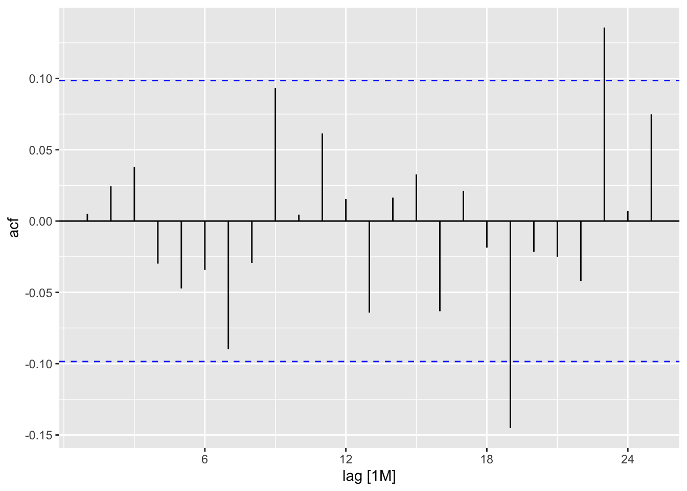
best.arima.elec[[3]][1] 0 1 1 2 0 2best_fit_elec# A mable: 1 x 1
ar_model
<model>
1 <ARIMA(2,0,1)(1,1,2)[12] w/ drift>ts.plot(cbind(window(Elec.ts,start = 1981),
exp(predict(best.fit.elec,12)$pred) ), lty = 1:2)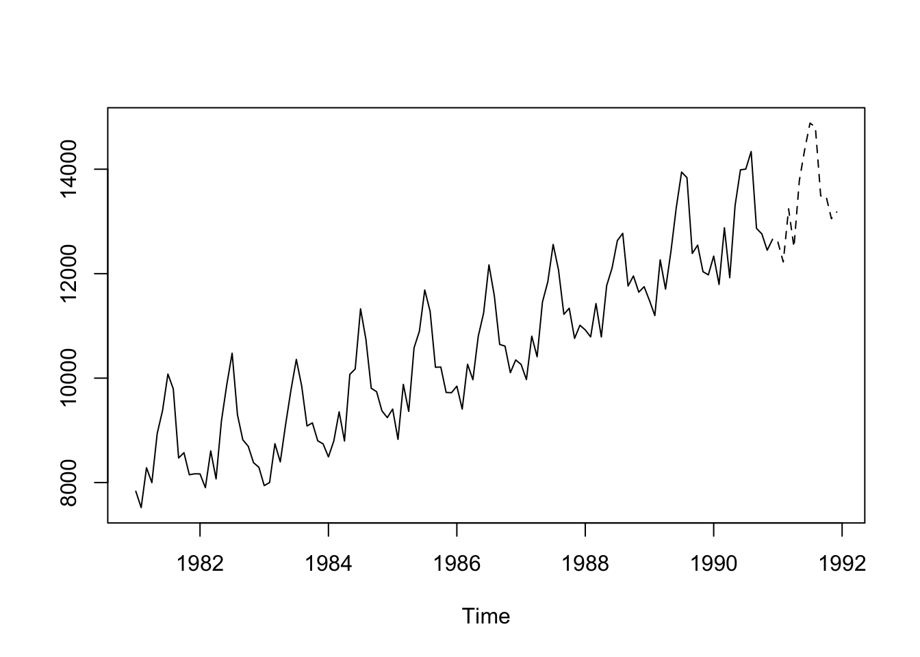
best_fit_elec |>
forecast(h = "12 months") |>
autoplot(filter(elec_ts, date > ymd("1981-01-01")))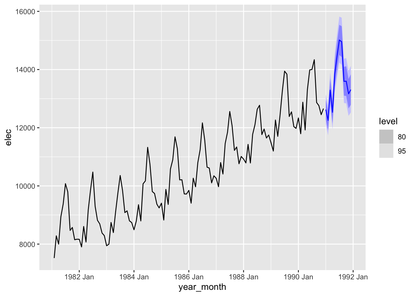
aic1 <- AIC(arima(log(Elec.ts),
order = c(1,1,0),
seas = list(order = c(1,0,0), 12)))
aic2 <- AIC(arima(log(Elec.ts),
order = c(0,1,1),
seas = list(order = c(0,0,1), 12)))
c("aic1" = aic1, "aic2" = aic2)
get.best.arima <- function(x.ts, maxord = c(1,1,1,1,1,1)) {
best.aic <- 1e8
n <- length(x.ts)
for (p in 0:maxord[1]) for(d in 0:maxord[2]) for(q in 0:maxord[3])
for (P in 0:maxord[4]) for(D in 0:maxord[5]) for(Q in 0:maxord[6])
{
fit <- arima(x.ts, order = c(p,d,q),
seas = list(order = c(P,D,Q),
frequency(x.ts)), method = "CSS")
fit.aic <- -2 * fit$loglik + (log(n) + 1) * length(fit$coef)
print(paste(paste(c(p,d,q,P,D,Q), collapse = "-"), "AIC:", fit.aic))
if (fit.aic < best.aic)
{
best.aic <- fit.aic
best.fit <- fit
best.model <- c(p,d,q,P,D,Q)
}
}
list(best.aic, best.fit, best.model)
}
best.arima.elec <- get.best.arima(
log(Elec.ts),
maxord = c(2,2,2,2,2,2))
best.fit.elec <- best.arima.elec[[2]]
acf(resid(best.fit.elec))
best.arima.elec[[3]]
ts.plot(cbind(window(Elec.ts,start = 1981),
exp(predict(best.fit.elec,12)$pred) ), lty = 1:2)elec_ts |>
model(
ar_model = ARIMA(log(elec) ~ 1 +
pdq(1, 1, 0) +
PDQ(1, 0, 0)),
ma_model = ARIMA(log(elec) ~ 1 +
pdq(0, 1, 1) +
PDQ(0, 0, 1))) |>
glance() |>
pull(AIC)
best_fit_elec <- elec_ts |>
model(
ar_model = ARIMA(log(elec) ~ 1 +
pdq(0:2, 0:2, 0:2) +
PDQ(0:2, 0:2, 0:2), approximation = TRUE))
best_fit_elec |>
residuals() |>
ACF() |>
autoplot()
glance(best_fit_elec) |> pull(AIC)
best_fit_elec |>
  forecast(h = "12 months") |>
  autoplot(filter(elec_ts, date > ymd("1981-01-01")))
# Very Slow, but you can see all fits.
# get_arima <- function(p, d, q, P, D, Q, data = elec_ts) {
# model(data, arima = ARIMA(log(elec) ~ 1 +
# pdq(p, d, q) + PDQ(P, D, Q), approximation = TRUE))
# }
# get_aic <- function(fit) {
# gfit <- glance(fit)
# if (nrow(gfit) != 0) {
# pull(gfit, AIC)
# } else {
# NA
# }
# }
# all_possible <- expand_grid(
# p = 0:2, d = 0:2, q = 0:2,
# P = 0:2, D = 0:2, Q = 0:2)
# all_possible <- all_possible |>
# mutate(
# fit = purrr::pmap(all_possible, get_arima),
# aic = purrr::map_dbl(fit, ~get_aic(.x))
# )
# filter(all_possible, aic == min(aic, na.rm = TRUE))Book code
library(MASS)
data(SP500)
plot(SP500, type = 'l')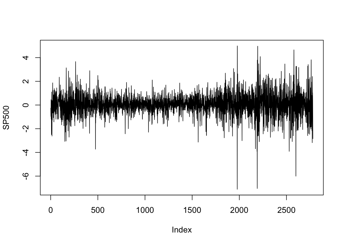
Tidyverts code
library(MASS)
data(SP500)
dat <- tibble(x = SP500) |>
  mutate(
    sq_mean_diff = (x - mean(x))^2,
    index = 1:n()) |>
  as_tsibble(index = index)
autoplot(dat)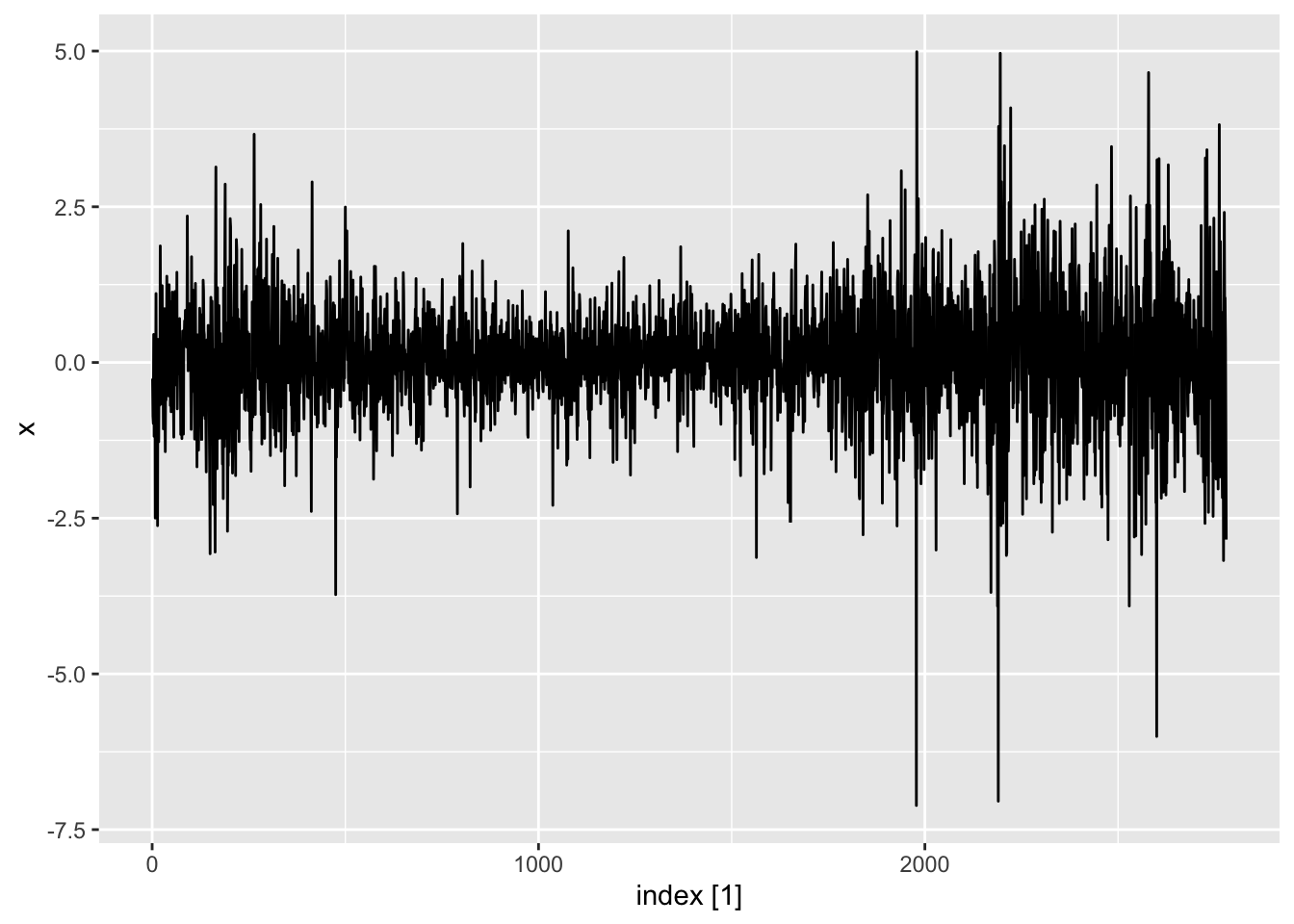
acf(SP500)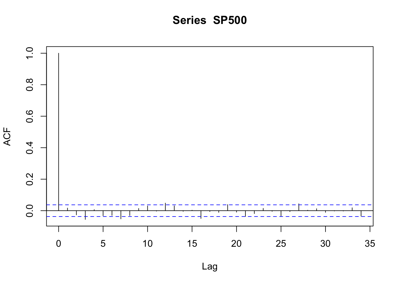
ACF(dat) |> autoplot()
acf((SP500 - mean(SP500))^2)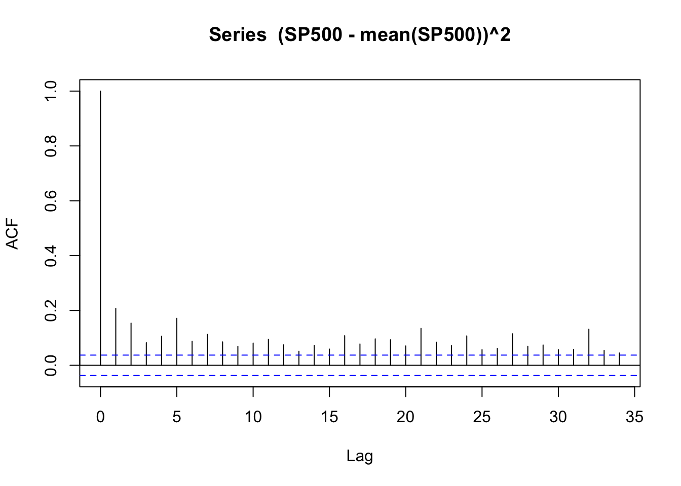
ACF(dat, y = sq_mean_diff) |> autoplot()
Book code
library(tseries)
set.seed(1)
alpha0 <- 0.1
alpha1 <- 0.4
beta1 <- 0.2
w <- rnorm(10000)
a <- rep(0, 10000)
h <- rep(0, 10000)
for (i in 2:10000) {
  h[i] <- alpha0 + alpha1 * (a[i - 1]^2) + beta1 * h[i - 1]
  a[i] <- w[i] * sqrt(h[i])
  }
acf(a)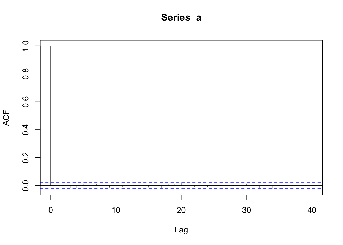
Tidyverts code
pacman::p_load("rugarch")
set.seed(1)
sim <- tibble(
  alpha0 = 0.1,
  alpha1 = 0.4,
  beta1 = 0.2,
  w = rnorm(10000),
  a = rep(0, 10000),
  h = rep(0, 10000)) |>
  mutate(index = 1:n()) |>
  as_tsibble(index = index)

for (i in 2:10000) {
  sim$h[i] <- sim$alpha0[1] + sim$alpha1[1] * (sim$a[i - 1]^2) + sim$beta1[1] * sim$h[i - 1]
  sim$a[i] <- sim$w[i] * sqrt(sim$h[i])
  }
sim <- mutate(sim, a2 = a^2)

ACF(sim, y = a) |>
  autoplot()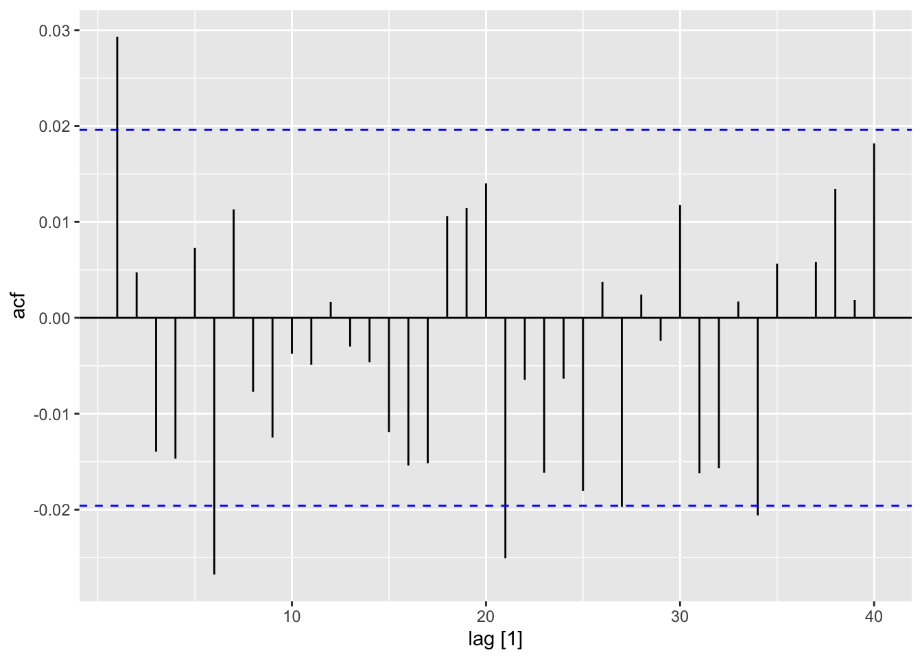
acf(a^2)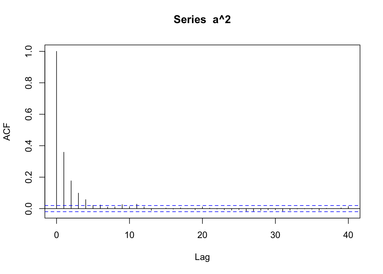
ACF(sim, y = a2) |>
  autoplot()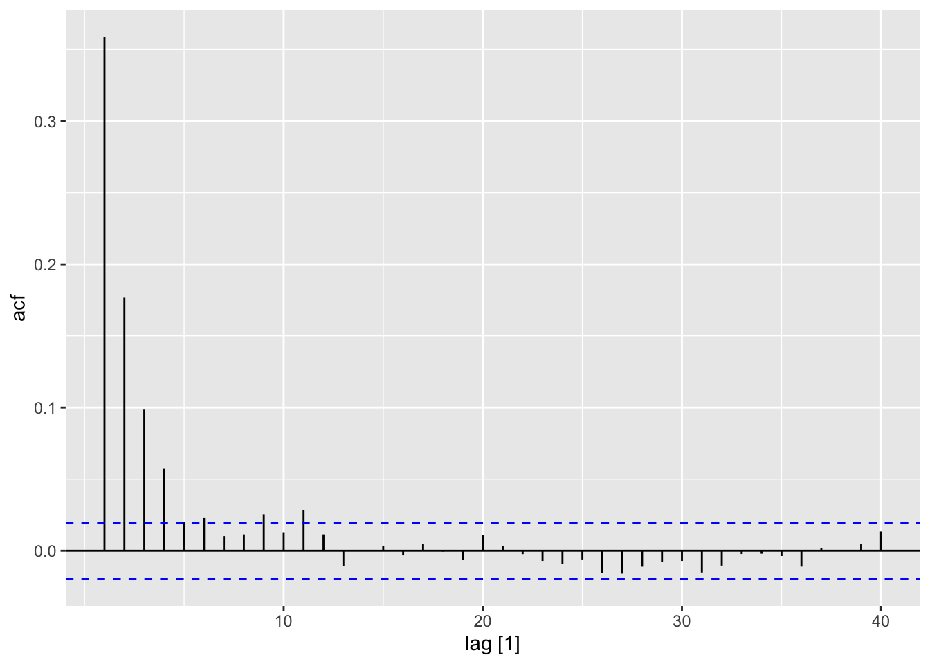
a.garch <- garch(a, grad = "numerical", trace = FALSE)
confint(a.garch)
2.5 % 97.5 %
a0 0.0882393 0.1092903
a1 0.3307897 0.4023932
b1 0.1928344 0.2954660spec <- ugarchspec(
mean.model = list(armaOrder = c(0,0)),
variance.model = list(model = "sGARCH"),
distribution.model = "norm")
sim_garch <- ugarchfit(data = pull(sim,a), spec = spec)
confint(sim_garch) 2.5 % 97.5 %
mu -0.008260573 0.008253128
omega 0.088325823 0.109204574
alpha1 0.331527684 0.401653876
beta1 0.192934674 0.295362333library(tseries)
set.seed(1)
alpha0 <- 0.1
alpha1 <- 0.4
beta1 <- 0.2
w <- rnorm(10000)
a <- rep(0, 10000)
h <- rep(0, 10000)
for (i in 2:10000) {
h[i] <- alpha0 + alpha1 * (a[i - 1]^2) + beta1 * h[i - 1]
a[i] <- w[i] * sqrt(h[i])
}
acf(a)
acf(a^2)
a.garch <- garch(a, grad = "numerical", trace = FALSE)
confint(a.garch)pacman::p_load("rugarch")
set.seed(1)
sim <- tibble(
alpha0 = 0.1,
alpha1 = 0.4,
beta1 = 0.2,
w = rnorm(10000),
a = rep(0, 10000),
h = rep(0, 10000)) |>
mutate(index = 1:n()) |>
as_tsibble(index = index)
for (i in 2:10000) {
sim$h[i] <- sim$alpha0[1] + sim$alpha1[1] * (sim$a[i - 1]^2) + sim$beta1[1] * sim$h[i - 1]
sim$a[i] <- sim$w[i] * sqrt(sim$h[i])
}
sim <- mutate(sim, a2 = a^2)
ACF(sim, y = a) |>
autoplot()
ACF(sim, y = a2) |>
autoplot()
spec <- rurgarch::ugarchspec(
mean.model = list(armaOrder = c(0,0)),
variance.model = list(model = "sGARCH"),
distribution.model = "norm")
sim_garch <- ugarchfit(data = pull(sim,a), spec = spec)
confint(sim_garch)
# gd <- ugarchdistribution(garchfit, n.sim = 500, recursive = TRUE,
# recursive.length = 6000, recursive.window = 500, m.sim = 100,
# solver = 'hybrid')
#garchforecast <- ugarchforecast(fitORspec = garchfit, n.ahead = 5)Book code
sp.garch <- garch(SP500, trace = F)
sp.res   <- sp.garch$res[-1]
acf(sp.res)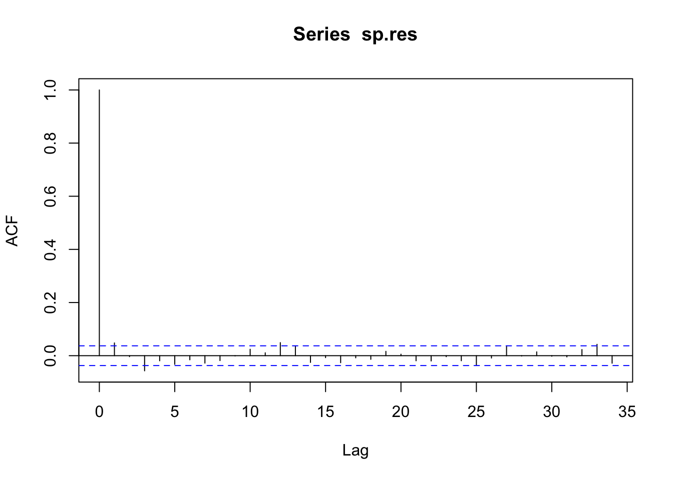
Tidyverts code
dat <- tibble::tibble(sp500 = SP500) |>
  mutate(index = 1:n()) |>
  as_tsibble(index = index)

spec <- ugarchspec(
    mean.model = list(armaOrder = c(0,0)),
    variance.model = list(model = "sGARCH"),
    distribution.model = "norm")

sp_garch <- ugarchfit(data = pull(dat, sp500), spec = spec)

dat <- dat |>
  mutate(
    .resid = residuals(sp_garch),
    .resid2 = .resid^2)

dat |>
  ACF(y = .resid) |>
  autoplot()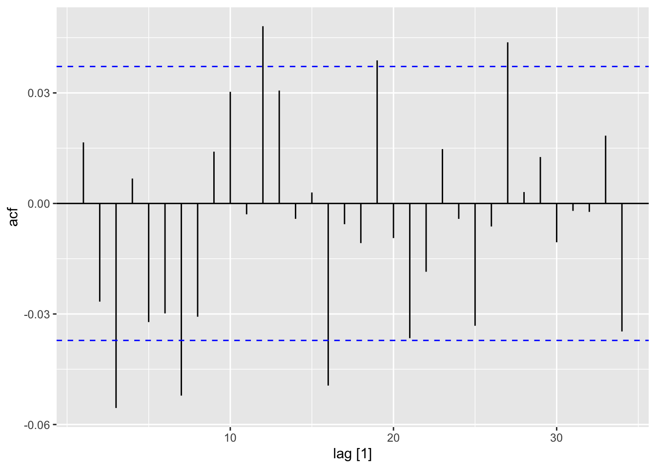
acf(sp.res^2)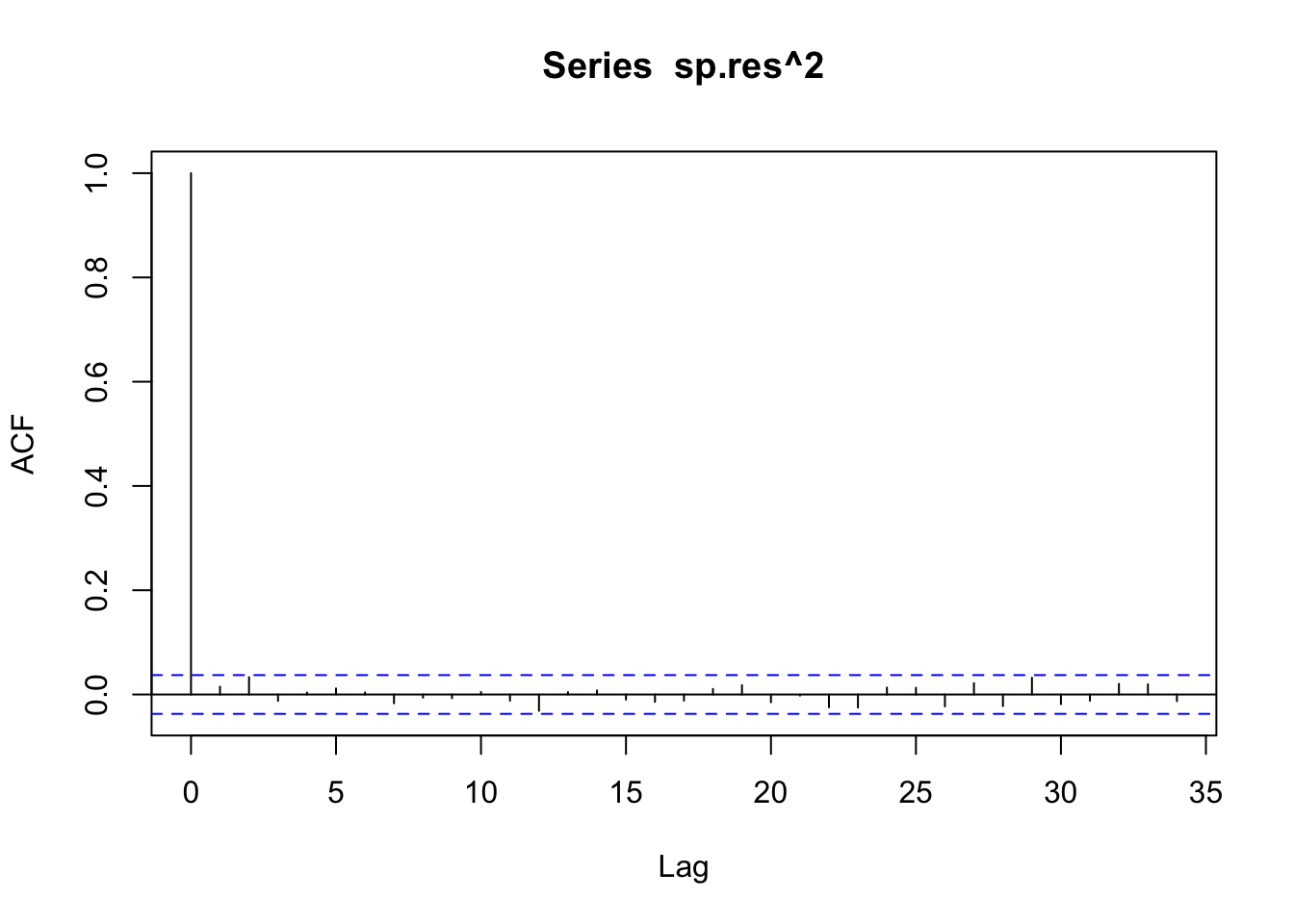
dat |>
  ACF(y = .resid2) |>
  autoplot()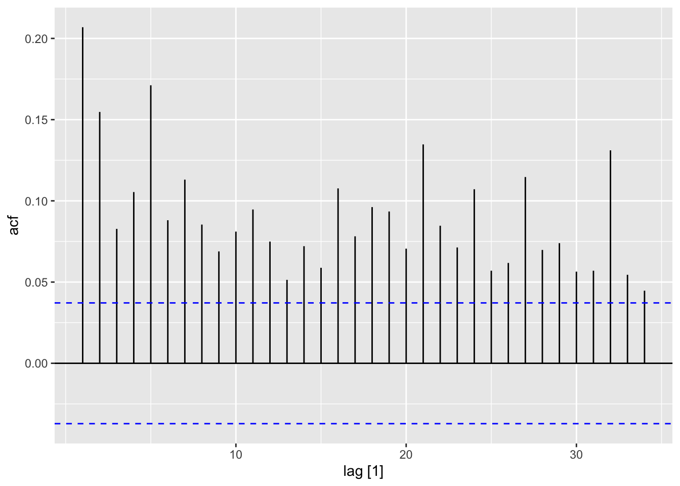
dat <- tibble::tibble(sp500 = SP500) |>
  mutate(index = 1:n()) |>
  as_tsibble(index = index)

spec <- ugarchspec(
    mean.model = list(armaOrder = c(0,0)),
    variance.model = list(model = "sGARCH"),
    distribution.model = "norm")

sp_garch <- ugarchfit(data = pull(dat, sp500), spec = spec)

dat <- dat |>
  mutate(
    .resid = residuals(sp_garch),
    .resid2 = .resid^2)

dat |>
  ACF(y = .resid) |>
  autoplot()

dat |>
  ACF(y = .resid2) |>
autoplot()Book code
stemp <- scan("data/stemp.dat")
stemp.ts <- ts(stemp, start = 1850, freq = 12)
plot(stemp.ts)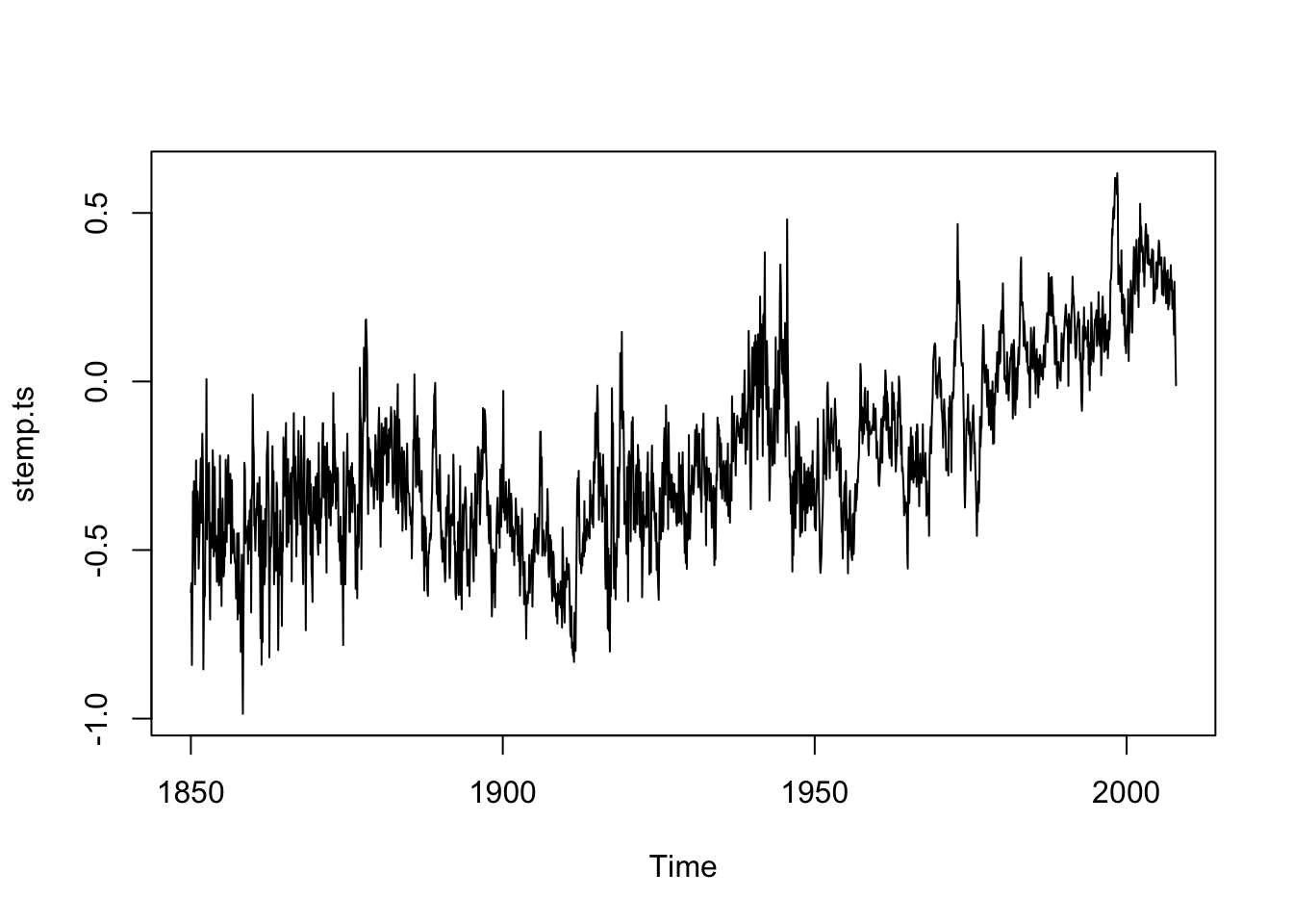
stemp.best <- get.best.arima(stemp.ts, maxord = rep(2,6))
stemp.best[[3]]
[1] 1 1 2 2 0 1stemp.arima <- arima(stemp.ts, order = c(1,1,2),
seas = list(order = c(2,0,1), 12))
t(confint(stemp.arima)) ar1 ma1 ma2 sar1 sar2 sma1
2.5 % 0.8317390 -1.447400 0.3256700 0.8576802 -0.02501883 -0.9690534
97.5 % 0.9127946 -1.312553 0.4530475 1.0041396 0.07413424 -0.8507034Tidyverts code
stemp_ts <- tibble::tibble(stemp = scan("data/stemp.dat")) |>
mutate(
date = seq(
ymd("1850-01-01"),
by = "1 months",
length.out = n()),
year_month = tsibble::yearmonth(date)) |>
as_tsibble(index = year_month)
autoplot(stemp_ts)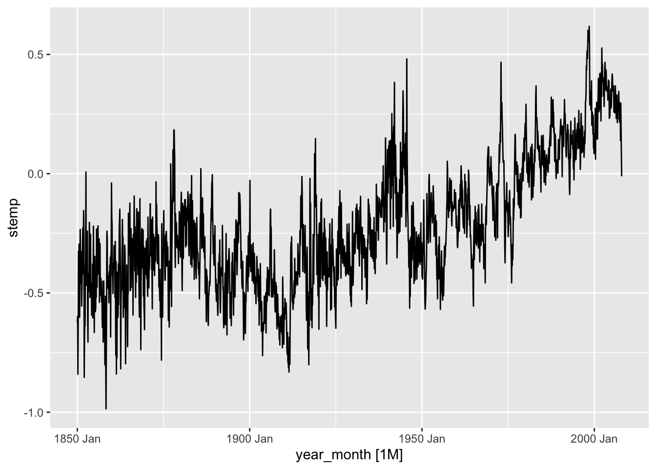
stemp_best <- stemp_ts |>
model(
ar_model = ARIMA(stemp ~ 1 +
pdq(0:2, 0:2, 0:2) +
PDQ(0:2, 0:2, 0:2), approximation = TRUE),
book_arima = ARIMA(stemp ~ 1 +
pdq(1, 1, 2) +
PDQ(2, 0, 1), approximation = TRUE),
book_arima_reduced = ARIMA(stemp ~ 1 +
pdq(1, 1, 2) +
PDQ(1, 0, 1), approximation = TRUE),
)
tidy(stemp_best) |>
dplyr::filter(term != "constant") |>
mutate(
lb = round(estimate + qnorm(.025) * std.error, 3),
ub = round(estimate + qnorm(.975) * std.error, 3),
interval = paste0(lb, " , ", ub)
) |>
dplyr::select(.model, term, interval) |>
pivot_wider(names_from = .model, values_from = interval, values_fill = "-") |>
knitr::kable()| term | ar_model | book_arima | book_arima_reduced |
|---|---|---|---|
| ar1 | 0.449 , 0.546 | 0.838 , 0.917 | 0.835 , 0.913 |
| ar2 | 0.161 , 0.257 | - | - |
| ma1 | -0.99 , -0.954 | -1.452 , -1.319 | -1.45 , -1.317 |
| sar1 | -0.01 , 0.083 | 0.845 , 0.997 | 0.917 , 0.995 |
| sar2 | -0.028 , 0.065 | -0.023 , 0.077 | - |
| ma2 | - | 0.33 , 0.456 | 0.328 , 0.454 |
| sma1 | - | -0.964 , -0.837 | -0.968 , -0.859 |
stemp.arima <- arima(stemp.ts, order = c(1,1,2),
seas = list(order = c(1,0,1), 12))
t(confint(stemp.arima)) ar1 ma1 ma2 sar1 sma1
2.5 % 0.8303969 -1.445048 0.3242572 0.9243526 -0.9694910
97.5 % 0.9108148 -1.311229 0.4508903 0.9956640 -0.8679276tidy(stemp_best) |>
dplyr::filter(term != "constant") |>
mutate(
lb = round(estimate + qnorm(.025) * std.error, 3),
ub = round(estimate + qnorm(.975) * std.error, 3),
interval = paste0(lb, " , ", ub)
) |>
dplyr::select(.model, term, interval) |>
pivot_wider(names_from = .model, values_from = interval, values_fill = "-") |>
knitr::kable()| term | ar_model | book_arima | book_arima_reduced |
|---|---|---|---|
| ar1 | 0.449 , 0.546 | 0.838 , 0.917 | 0.835 , 0.913 |
| ar2 | 0.161 , 0.257 | - | - |
| ma1 | -0.99 , -0.954 | -1.452 , -1.319 | -1.45 , -1.317 |
| sar1 | -0.01 , 0.083 | 0.845 , 0.997 | 0.917 , 0.995 |
| sar2 | -0.028 , 0.065 | -0.023 , 0.077 | - |
| ma2 | - | 0.33 , 0.456 | 0.328 , 0.454 |
| sma1 | - | -0.964 , -0.837 | -0.968 , -0.859 |
stemp.res <- resid(stemp.arima)
layout(1:2)
acf(stemp.res)
acf(stemp.res^2)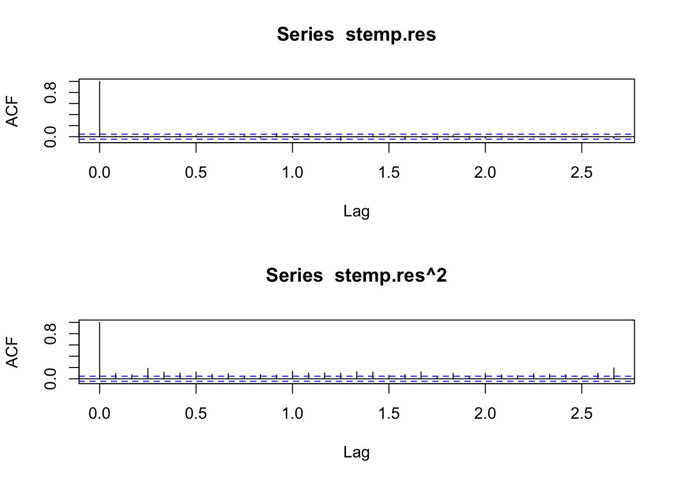
stemp_res <- stemp_best |>
dplyr::select(book_arima_reduced) |>
residuals() |>
mutate(.resid2 = .resid^2)
rp <- ACF(stemp_res, y = .resid) |> autoplot()
r2p <- ACF(stemp_res, y = .resid2) |> autoplot()
rp / r2p
stemp.garch <- garch(stemp.res, trace = F)
confint(stemp.garch) 2.5 % 97.5 %
a0 1.064246e-05 0.0001485812
a1 3.299179e-02 0.0652567733
b1 9.249316e-01 0.9630787389spec <- ugarchspec(
mean.model = list(armaOrder = c(0,0)),
variance.model = list(model = "sGARCH"),
distribution.model = "norm")
stemp_garch <- ugarchfit(data = pull(stemp_res, .resid), spec = spec)
confint(stemp_garch) 2.5 % 97.5 %
mu -3.974225e-03 0.0044798310
omega 2.246930e-06 0.0001533503
alpha1 2.884755e-02 0.0691398769
beta1 9.215237e-01 0.9670927847stemp.garch.res <- resid(stemp.garch)[-1]
layout(1:2)
acf(stemp.garch.res)
acf(stemp.garch.res^2)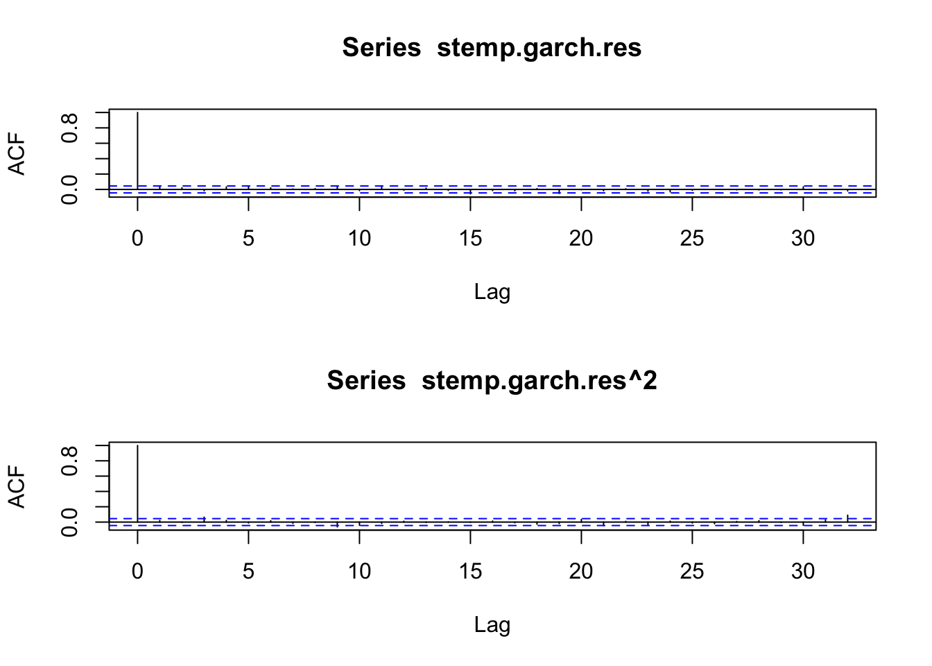
stemp_res <- stemp_res |>
mutate(
.resid_garch = residuals(stemp_garch),
.resid2_garch = .resid_garch^2)
rgp <- ACF(stemp_res, y = .resid_garch) |> autoplot()
rg2p <- ACF(stemp_res, y = .resid2_garch) |> autoplot()
rgp / rg2p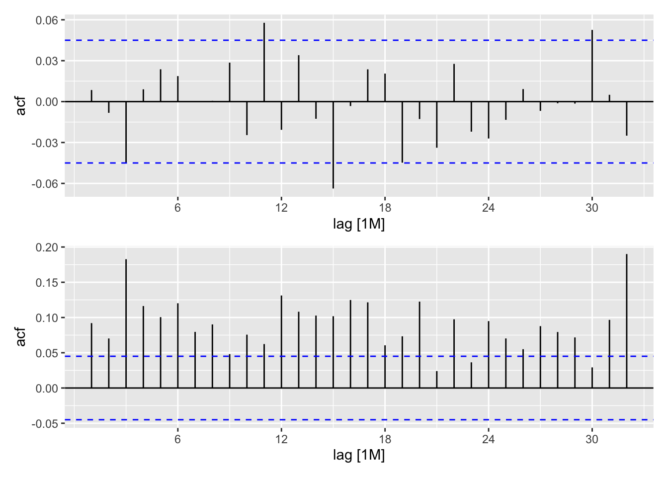
stemp <- scan("data/stemp.dat")
stemp.ts <- ts(stemp, start = 1850, freq = 12)
plot(stemp.ts)
stemp.best <- get.best.arima(stemp.ts, maxord = rep(2,6))
stemp.best[[3]]
stemp.arima <- arima(stemp.ts, order = c(1,1,2),
  seas = list(order = c(2,0,1), 12))
t(confint(stemp.arima))
stemp.arima <- arima(stemp.ts, order = c(1,1,2),
seas = list(order = c(1,0,1), 12))
t(confint(stemp.arima))
stemp.res <- resid(stemp.arima)
layout(1:2)
acf(stemp.res)
acf(stemp.res^2)
stemp.garch <- garch(stemp.res, trace = F)
confint(stemp.garch)
stemp.garch.res <- resid(stemp.garch)[-1]
acf(stemp.garch.res)
acf(stemp.garch.res^2)stemp_ts <- tibble::tibble(stemp = scan("data/stemp.dat")) |>
mutate(
date = seq(
ymd("1850-01-01"),
by = "1 months",
length.out = n()),
year_month = tsibble::yearmonth(date)) |>
as_tsibble(index = year_month)
autoplot(stemp_ts)
stemp_best <- stemp_ts |>
  model(
    ar_model = ARIMA(stemp ~ 1 +
      pdq(0:2, 0:2, 0:2) +
      PDQ(0:2, 0:2, 0:2), approximation = TRUE),
    book_arima = ARIMA(stemp ~ 1 +
      pdq(1, 1, 2) +
      PDQ(2, 0, 1), approximation = TRUE),
    book_arima_reduced = ARIMA(stemp ~ 1 +
      pdq(1, 1, 2) +
      PDQ(1, 0, 1), approximation = TRUE),
      )

tidy(stemp_best) |>
  dplyr::filter(term != "constant") |>
  mutate(
    lb = round(estimate + qnorm(.025) * std.error, 3),
    ub = round(estimate + qnorm(.975) * std.error, 3),
    interval = paste0(lb, " , ", ub)
  ) |>
  dplyr::select(.model, term, interval) |>
  pivot_wider(names_from = .model, values_from = interval, values_fill = "-") |>
  knitr::kable()
stemp_res <- stemp_best |>
dplyr::select(book_fit_reduced) |>
residuals() |>
mutate(.resid2 = .resid^2)
rp <- ACF(stemp_res, y = .resid) |> autoplot()
r2p <- ACF(stemp_res, y = .resid2) |> autoplot()
rp / r2p
spec <- ugarchspec(
    mean.model = list(armaOrder = c(0,0)),
    variance.model = list(model = "sGARCH"),
    distribution.model = "norm")

stemp_garch <- ugarchfit(data = pull(stemp_res, .resid), spec = spec)
confint(stemp_garch)
stemp.garch <- garch(stemp.res, trace = F)
t(confint(stemp.garch)
stemp_res <- stemp_res |>
  mutate(
    .resid_garch = residuals(stemp_garch),
    .resid2_garch = .resid_garch^2)

rgp <- ACF(stemp_res, y = .resid_garch) |> autoplot()
rg2p <- ACF(stemp_res, y = .resid2_garch) |> autoplot()
rgp / rg2pR commands used in examplesrugarch::ugarchspec(): Univariate GARCH Specificationrugarch::ugarchfit(): Univariate GARCH Fittingstats::confint(): Confidence Intervals for Model Parameters