Appendix

Dealing with missing time steps

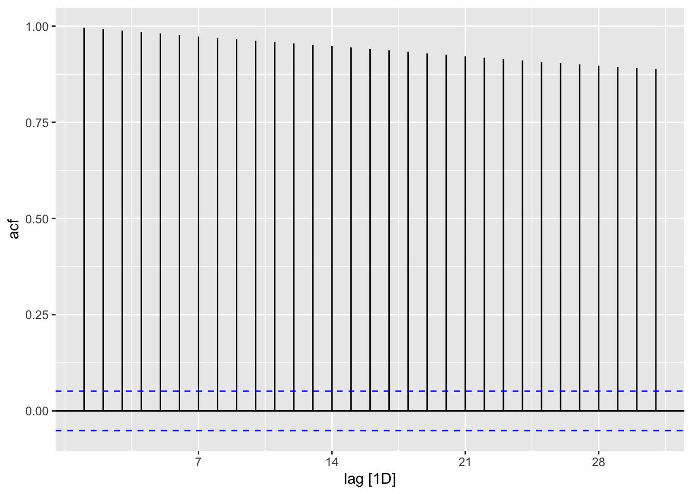
# https://stackoverflow.com/questions/72332262/forecasting-irregular-stock-data-with-arima-and-tsibble
pacman::p_load("tidyquant", "tsibble", "fable", "feasts",
    "tsibbledata", "fable.prophet", "tidyverse")
# Set symbol and date range
symbol <- "MCD"
company <- "McDonald's"
date_start <- "2020-01-01"
date_end <- "2024-01-01"

# Fetch stock prices (can be used to get new data)
stock_df <- tq_get(symbol, from = date_start, to = date_end, get = "stock.prices")

# Transform data into tibble
stock_ts <- stock_df |>
    select(date, adjusted) |>
    rename(value = adjusted) |>
    tsibble(index = date, regular = TRUE) |>
    fill_gaps() |>
    tidyr::fill(value, .direction = "down") |>
    mutate(diff = value - lag(value))


stock_ts |>
ACF(var = value) |>
autoplot()

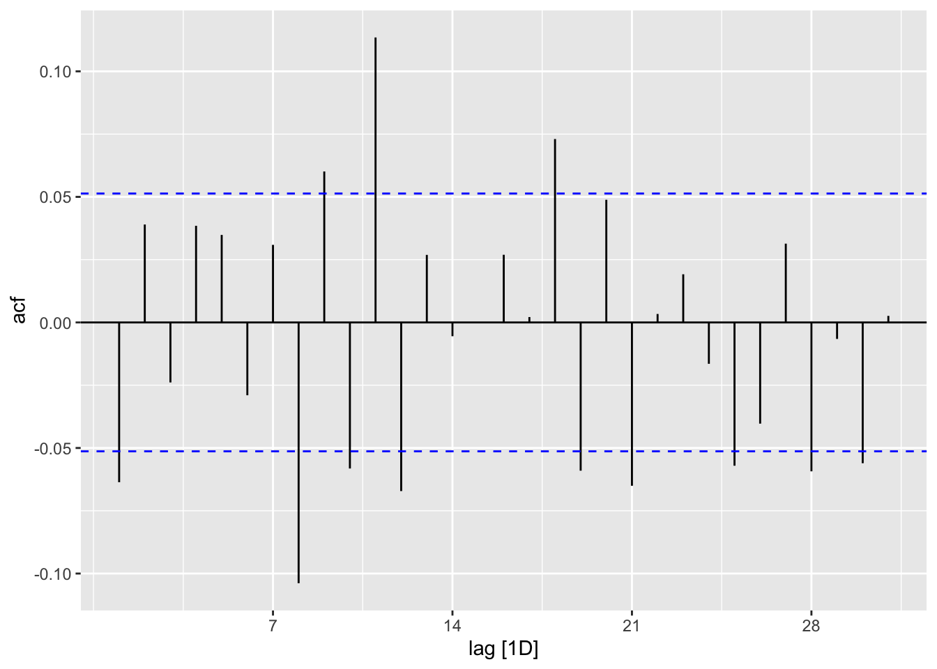
stock_ts |>
ACF(var = diff) |>
autoplot()

# acf(stock_ts$value, plot=TRUE, type = "correlation", lag.max = 25)

Intercept model

pacman::p_load("tidyquant", "tsibble", "fable", "feasts",
    "tsibbledata", "fable.prophet", "tidyverse")
set.seed(123)
n_rep <- 1000
alpha1 <- 0.75

dat_ts <- tibble(w = rnorm(n_rep)) |>
  mutate(
    index = 1:n(),
    x = purrr::accumulate2(
      lag(w), w, 
      \(acc, nxt, w) alpha1 * acc + w,
      .init = 0)[-1]) |>
  tsibble::as_tsibble(index = index)

fit_ar <- dat_ts |>
  model(AR(x ~ 1 + order(1)))
tidy(fit_ar)

# A tibble: 2 × 6
  .model               term     estimate std.error statistic   p.value
  <chr>                <chr>       <dbl>     <dbl>     <dbl>     <dbl>
1 AR(x ~ 1 + order(1)) constant   0.0188    0.0314     0.600 5.49e-  1
2 AR(x ~ 1 + order(1)) ar1        0.719     0.0220    32.7   5.95e-160

2nd Order AR Model Sims

set.seed(123)
n_rep <- 1000
alpha0 <- 20
alpha1 <- 0.5
alpha2 <- 0.4

dat_ts <- tibble(w = rnorm(n_rep)) |>
    mutate(
      index = 1:n(),
      x = 0
    ) |>
    tsibble::as_tsibble(index = index)

# Simulate x values
dat_ts$x[1] <- alpha0 + dat_ts$w[1]
dat_ts$x[2] <- alpha0 + alpha1 * ( dat_ts$x[1] - alpha0 ) + dat_ts$w[2]
for (i in 3:nrow(dat_ts)) {
  dat_ts$x[i] <- alpha0 + 
    alpha1 * ( dat_ts$x[i-1] - alpha0 ) + 
    alpha2 * ( dat_ts$x[i-2] - alpha0 ) + 
    dat_ts$w[i]
}

dat_ts |> 
  autoplot(.vars = x) +
    labs(
      x = "Time",
      y = "Simulated Time Series",
      title = paste("Simulated Values from an AR(2) Process with Mean", alpha0)
    ) +
    theme_minimal() +
    theme(
      plot.title = element_text(hjust = 0.5)
    )

# https://arc.net/l/quote/wuzdpjul
set.seed(123) # this doesn't seem to affect the starting point in arima.sim
n_rep <- 1000
alpha0 <- 20
alpha1 <- 0.5
alpha2 <- 0.4
drift <- 0.2
sigma <- 1

dat_ts2 <- tibble(x = alpha0 + arima.sim(
    list(ar = c(alpha1, alpha2)),
    n = n_rep,
    sd = sigma)) |>
    mutate(index = 1:n()) |>
    tsibble::as_tsibble(index = index)

dat_ts2 |> 
  autoplot(.vars = x) +
    labs(
      x = "Time",
      y = "Simulated Time Series",
      title = paste("Simulated Values from an AR(2) Process with Mean", alpha0)) +
    theme_minimal() +
    theme(plot.title = element_text(hjust = 0.5))

# xtWithDrift <- xt + drift * seq(1, n_rep)
# https://arc.net/l/quote/hznvagdn
# https://arc.net/l/quote/wuzdpjul
dat_ts |>
    model(AR(x ~ order(1:6))) |>
    tidy()

# A tibble: 3 × 6
  .model             term     estimate std.error statistic  p.value
  <chr>              <chr>       <dbl>     <dbl>     <dbl>    <dbl>
1 AR(x ~ order(1:6)) constant    2.29     0.363       6.32 3.94e-10
2 AR(x ~ order(1:6)) ar1         0.478    0.0289     16.5  1.75e-54
3 AR(x ~ order(1:6)) ar2         0.408    0.0289     14.1  1.96e-41

dat_ts2 |>
    model(AR(x ~ order(1:6))) |>
    tidy()

# A tibble: 3 × 6
  .model             term     estimate std.error statistic  p.value
  <chr>              <chr>       <dbl>     <dbl>     <dbl>    <dbl>
1 AR(x ~ order(1:6)) constant    2.22     0.358       6.21 7.86e-10
2 AR(x ~ order(1:6)) ar1         0.479    0.0289     16.6  9.54e-55
3 AR(x ~ order(1:6)) ar2         0.411    0.0289     14.2  4.80e-42