In most branches of science, engineering, and commerce, there are variables measured sequentially in time. Reserve banks record interest rates and exchange rates each day. The government statistics department will compute the country’s gross domestic product on a yearly basis. Newspapers publish yesterday’s noon temperatures for capital cities from around the world. Meteorological offices record rainfall at many different sites with differing resolutions. When a variable is measured sequentially in time over or at a fixed interval, known as the sampling interval , the resulting data form a time series .
We can use varied methods on the AP R object which is of the class ts which is an abbreviation for matrix of a ‘time series’ format. It is not a data.frame or a tibble as you have seen in your previous R courses. The base plot() function has a plotting method for ts data objects. Within the tidyverts we can use autoplot() to create default plots on our tsibble objects.
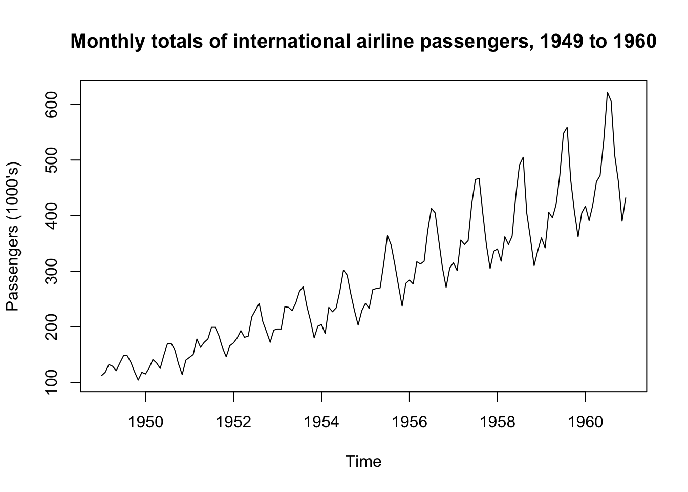
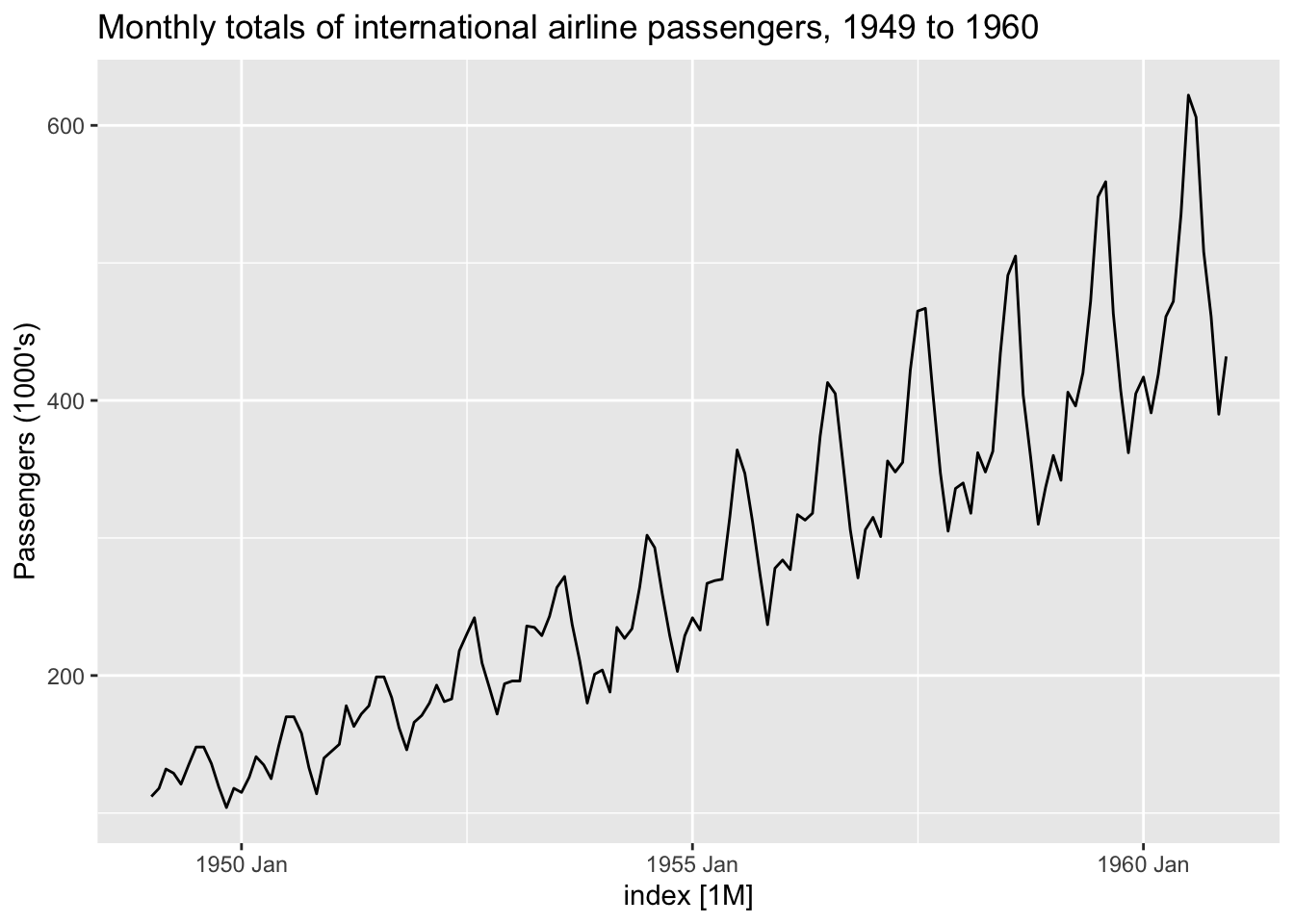
1.4.1 ‘A flying start: Air passenger bookings’ Modern Look
Book code
data (AirPassengers)<- AirPassengers
     Jan Feb Mar Apr May Jun Jul Aug Sep Oct Nov Dec
1949 112 118 132 129 121 135 148 148 136 119 104 118
1950 115 126 141 135 125 149 170 170 158 133 114 140
1951 145 150 178 163 172 178 199 199 184 162 146 166
1952 171 180 193 181 183 218 230 242 209 191 172 194
1953 196 196 236 235 229 243 264 272 237 211 180 201
1954 204 188 235 227 234 264 302 293 259 229 203 229
1955 242 233 267 269 270 315 364 347 312 274 237 278
1956 284 277 317 313 318 374 413 405 355 306 271 306
1957 315 301 356 348 355 422 465 467 404 347 305 336
1958 340 318 362 348 363 435 491 505 404 359 310 337
1959 360 342 406 396 420 472 548 559 463 407 362 405
1960 417 391 419 461 472 535 622 606 508 461 390 432
Tidyverts code
# install.packages("pacman") :: p_load ("tsibble" , "fable" , "feasts" ,"tsibbledata" , "fable.prophet" , "tidyverse" , "patchwork" )<- as_tsibble (AirPassengers) |> mutate (Year = year (index),Month = month (index)
# A tsibble: 144 x 4 [1M]
      index value  Year Month
      <mth> <dbl> <dbl> <dbl>
 1 1949 Jan   112  1949     1
 2 1949 Feb   118  1949     2
 3 1949 Mar   132  1949     3
 4 1949 Apr   129  1949     4
 5 1949 May   121  1949     5
 6 1949 Jun   135  1949     6
 7 1949 Jul   148  1949     7
 8 1949 Aug   148  1949     8
 9 1949 Sep   136  1949     9
10 1949 Oct   119  1949    10
# ℹ 134 more rows
[1] "tbl_ts" "tbl_df" "tbl" "data.frame"
# A tsibble: 1 x 4 [1M]
     index value  Year Month
     <mth> <dbl> <dbl> <dbl>
1 1949 Jan   112  1949     1
# A tsibble: 1 x 4 [1M]
     index value  Year Month
     <mth> <dbl> <dbl> <dbl>
1 1960 Dec   432  1960    12
guess_frequency (ap$ index)
plot (AP, ylab = "Passengers (1000's)" ,main = "Monthly totals of international airline passengers, 1949 to 1960" )
autoplot (ap) + labs (y = "Passengers (1000's)" ,title = "Monthly totals of international airline passengers, 1949 to 1960"
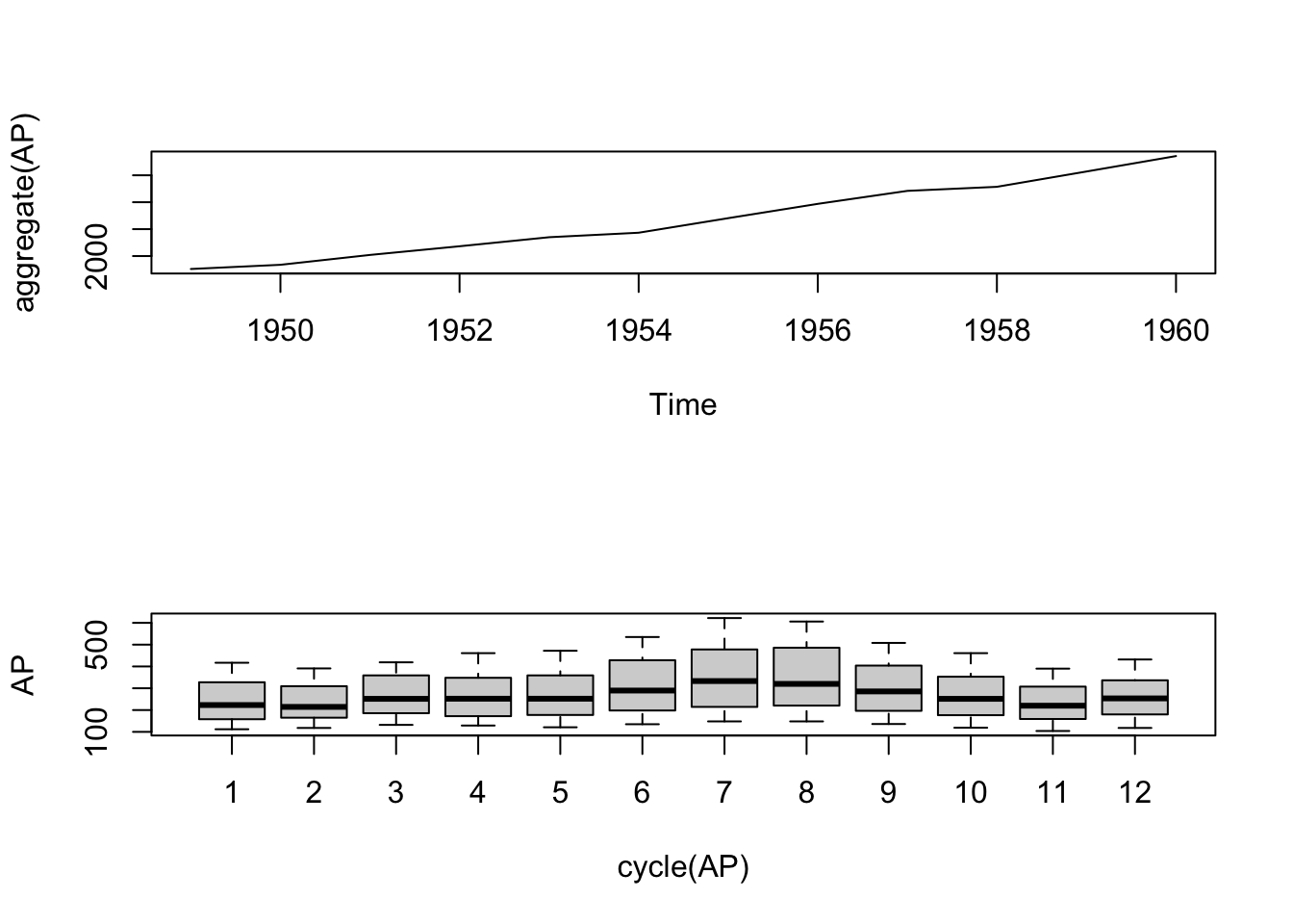
layout (1 : 2 )plot (aggregate (AP))boxplot (AP ~ cycle (AP))
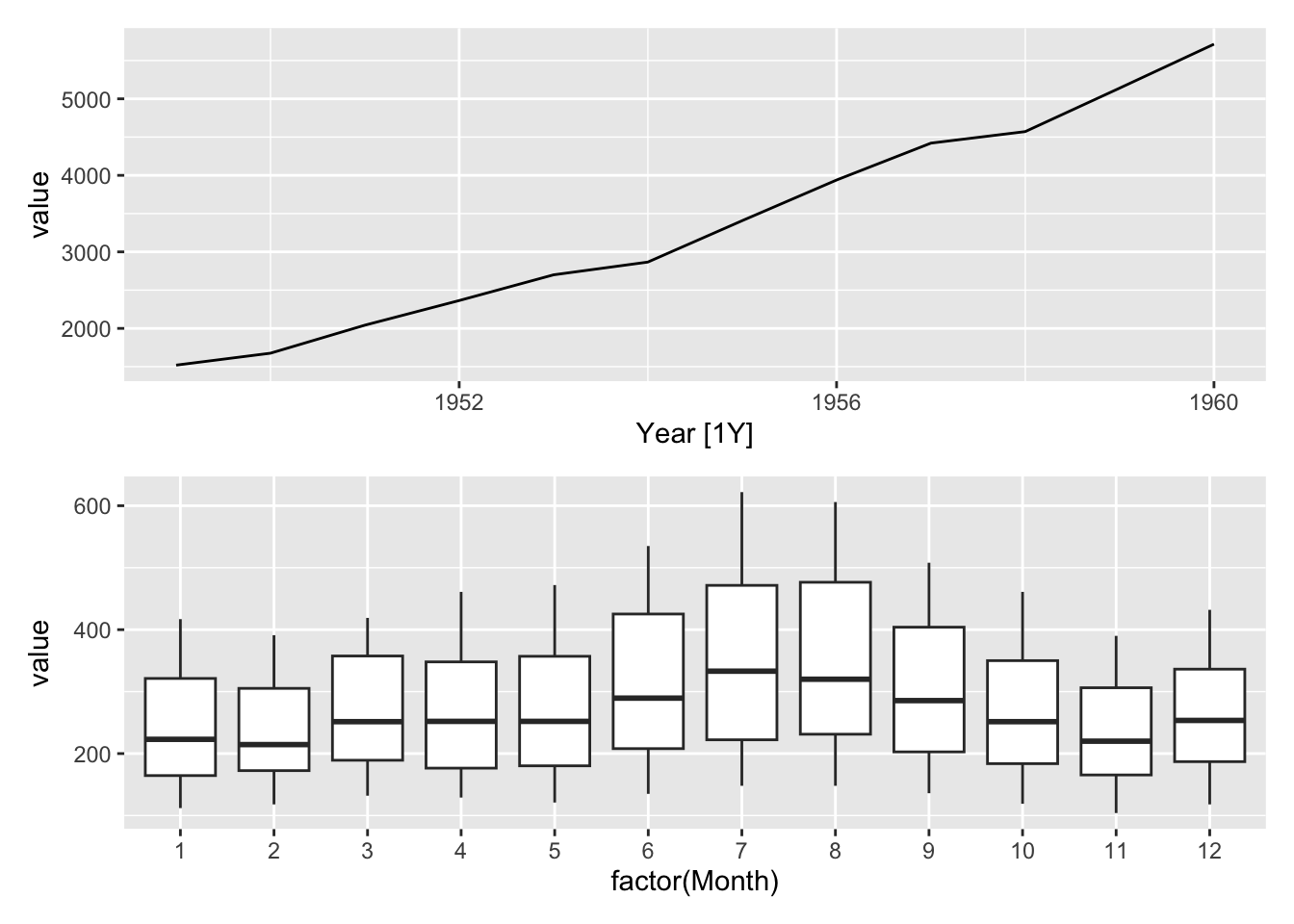
# pacman::p_load("patchwork") <- autoplot (summarise (index_by (ap, Year), value = sum (value)))<- ggplot (ap, aes (x = factor (Month), y = value)) + geom_boxplot ()/ pbox
Show the book code in full
data (AirPassengers)<- AirPassengersclass (AP)start (AP)end (AP)frequency (AP)plot (AP, ylab = "Passengers (1000's)" ,main = "Monthly totals of international airline passengers, 1949 to 1960" )layout (1 : 2 )plot (aggregate (AP))boxplot (AP ~ cycle (AP))
Show the Tidyverts code in full
data (AirPassengers)install.packages ("pacman" ):: p_load ("tsibble" , "fable" , "feasts" ,"tsibbledata" , "fable.prophet" , "tidyverse" , "patchwork" )<- as_tsibble (AirPassengers) |> mutate (Year = year (index),Month = month (index)class (ap)head (ap, 1 )tail (ap, 1 )guess_frequency (ap$ index)autoplot (ap) + labs (y = "Passengers (1000's)" ,title = "Monthly totals of international airline passengers, 1949 to 1960" <- autoplot (summarise (index_by (ap, Year), value = sum (value)))<- ggplot (ap, aes (x = factor (Month), y = value)) + geom_boxplot ()/ pbox
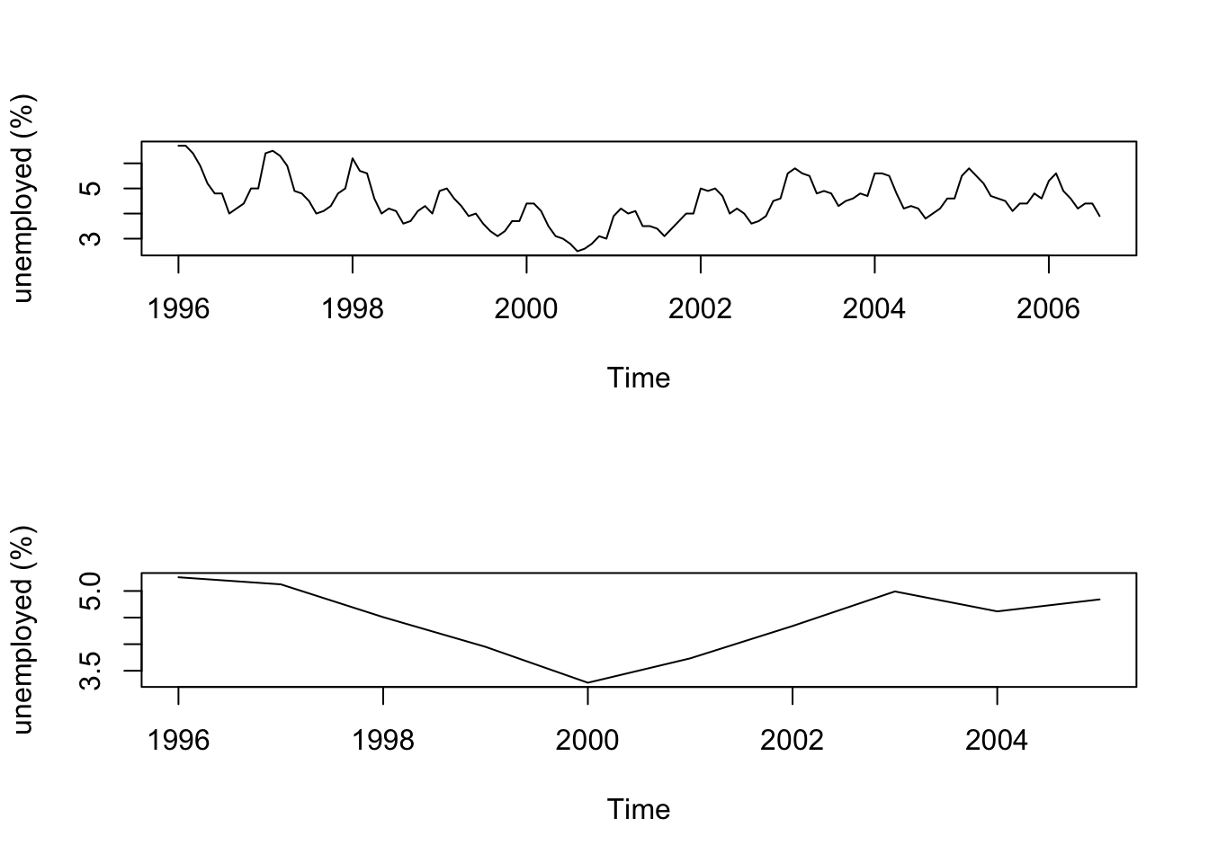
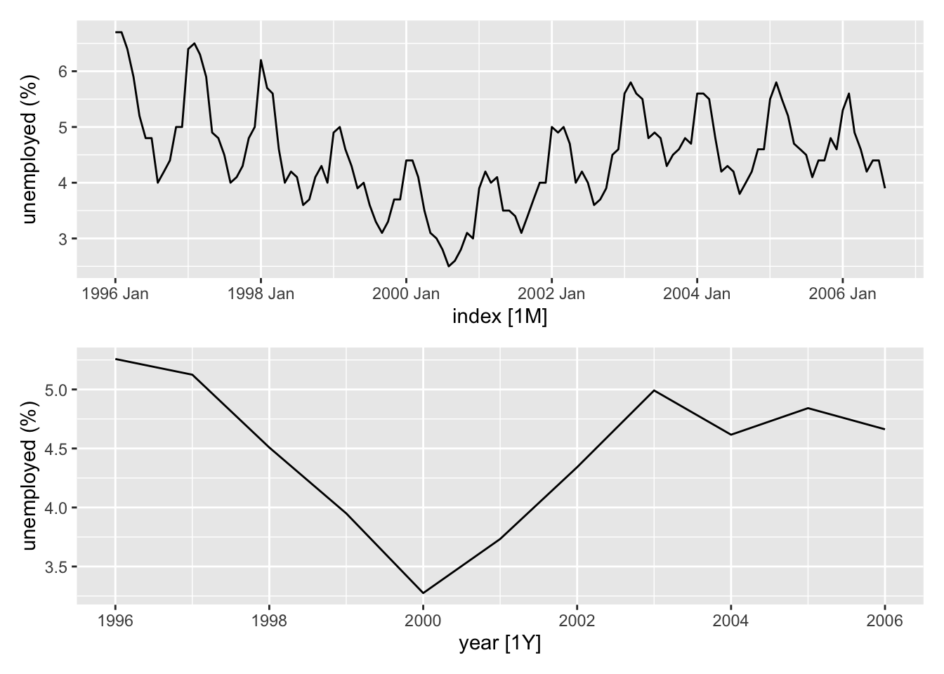
1.4.2 ‘Unemployment: Maine’ Modern Look
Note: The book uses attach() in their examples, a terrible practice (tp) in modern R programming. We have opted not to recreate their code exactly when using attach().
Book code
<- read.table ("data/Maine.dat" , header = TRUE )# attach(Maine.month) tp <- ts (Maine.month, start = c (1996 , 1 ), freq = 12 )<- aggregate (Maine.month.ts)/ 12
Time Series:
Start = 1996
End = 2005
Frequency = 1
      unemploy
 [1,] 5.258333
 [2,] 5.125000
 [3,] 4.508333
 [4,] 3.950000
 [5,] 3.275000
 [6,] 3.733333
 [7,] 4.341667
 [8,] 4.991667
 [9,] 4.616667
[10,] 4.841667
Tidyverts code
# install.packages("pacman") :: p_load ("tsibble" , "fable" , "feasts" , "tsibbledata" ,"fable.prophet" , "tidyverse" ,"patchwork" )<- read_table ("data/Maine.dat" )<- lubridate:: ymd ("1996-01-01" )<- seq (start_date,+ months (nrow (maine_month)- 1 ),by = "1 months" )<- tibble (dates = date_seq,year = lubridate:: year (date_seq),month = lubridate:: month (date_seq),value = pull (maine_month, unemploy)<- maine |> mutate (index = tsibble:: yearmonth (dates)) |> as_tsibble (index = index)<- summarise (index_by (maine_month_ts, year), value = mean (value))
# A tsibble: 11 x 2 [1Y]
    year value
   <dbl> <dbl>
 1  1996  5.26
 2  1997  5.12
 3  1998  4.51
 4  1999  3.95
 5  2000  3.28
 6  2001  3.73
 7  2002  4.34
 8  2003  4.99
 9  2004  4.62
10  2005  4.84
11  2006  4.66
layout (1 : 2 )plot (Maine.month.ts, ylab = "unemployed (%)" )plot (Maine.annual.ts, ylab = "unemployed (%)" )
<- autoplot (maine_month_ts, .vars = value) + labs (y = "unemployed (%)" )<- autoplot (maine_annual_ts) + labs (y = "unemployed (%)" ) + scale_x_continuous (breaks = seq (1900 , 2010 , by = 2 ))/ yp
<- window (Maine.month.ts, start = c (1996 ,2 ), freq = TRUE )<- window (Maine.month.ts, start = c (1996 ,8 ), freq = TRUE )<- mean (Maine.Feb) / mean (Maine.month.ts))<- mean (Maine.Aug) / mean (Maine.month.ts))
= filter (maine, month == 2 )= filter (maine, month == 8 )<- mean (pull (maine_feb, value)) / mean (pull (maine_month_ts, value)))<- mean (pull (maine_aug, value)) / mean (pull (maine_month_ts, value)))
Show the Book code in full
<- read.table ("data/Maine.dat" , header = TRUE )# attach(Maine.month) this is a bad deal class (Maine.month)<- ts (Maine.month, start = c (1996 , 1 ), freq = 12 )<- aggregate (Maine.month.ts)/ 12 layout (1 : 2 )plot (Maine.month.ts, ylab = "unemployed (%)" )plot (Maine.annual.ts, ylab = "unemployed (%)" )<- window (Maine.month.ts, start = c (1996 ,2 ), freq = TRUE )<- window (Maine.month.ts, start = c (1996 ,8 ), freq = TRUE )<- mean (Maine.Feb) / mean (Maine.month.ts))<- mean (Maine.Aug) / mean (Maine.month.ts))
Show the Tidyverts code in full
install.packages ("pacman" ):: p_load ("tsibble" , "fable" , "feasts" , "tsibbledata" ,"fable.prophet" , "tidyverse" , "patchwork" )<- read_table ("data/Maine.dat" )<- lubridate:: ymd ("1996-01-01" )<- seq (start_date,+ months (nrow (maine_month)- 1 ),by = "1 months" )<- tibble (dates = date_seq,year = lubridate:: year (date_seq),month = lubridate:: month (date_seq),value = pull (maine_month, unemploy)<- maine |> mutate (index = tsibble:: yearmonth (dates)) |> as_tsibble (index = index)<- summarise (index_by (maine_month_ts, year), value = mean (value))<- autoplot (maine_month_ts, .vars = value) + labs (y = "unemployed (%)" )<- autoplot (maine_annual_ts) + labs (y = "unemployed (%)" ) + scale_x_continuous (breaks = seq (1900 , 2010 , by = 2 ))/ yp= filter (maine, month == 2 )= filter (maine, month == 8 )<- mean (pull (maine_feb, value)) / mean (pull (maine_month_ts, value)))<- mean (pull (maine_aug, value)) / mean (pull (maine_month_ts, value)))
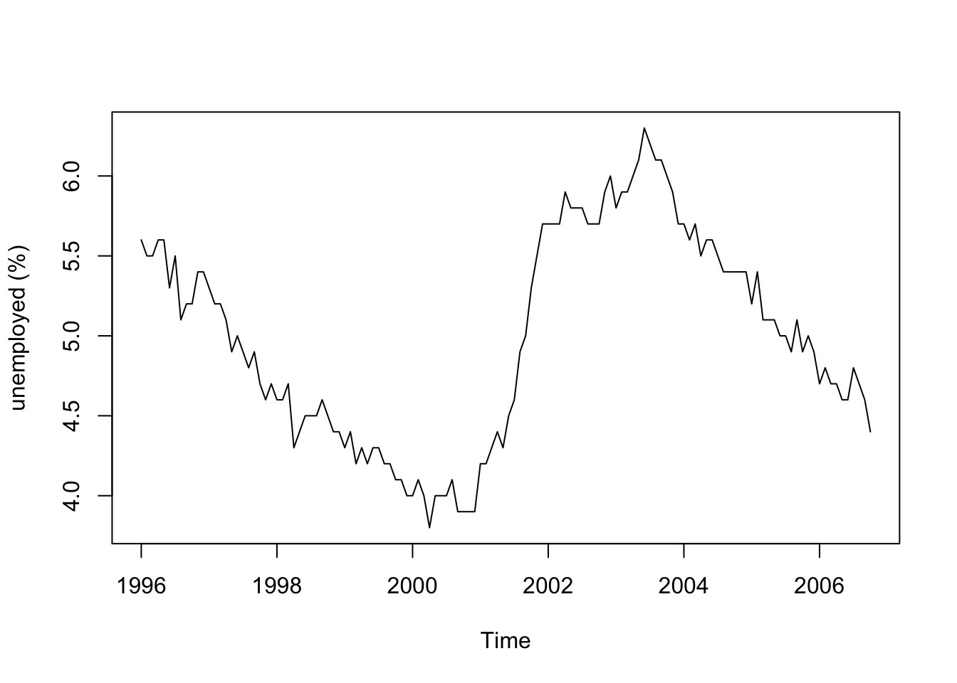
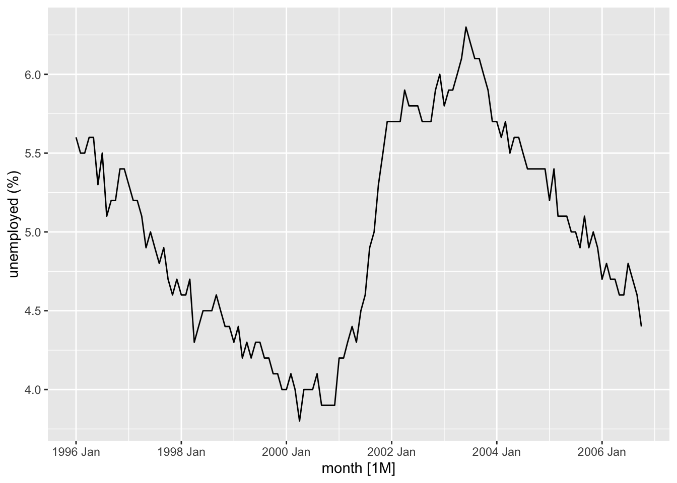
1.4.2 ‘US unemployment’ Modern Look
Book code
<- read.table ("data/USunemp.dat" , header = T)# attach(US.month) tp <- ts (US.month$ USun, start= c (1996 ,1 ), end= c (2006 ,10 ), freq = 12 )plot (US.month.ts, ylab = "unemployed (%)" )
Tidyverts code
<- read_table ("data/USunemp.dat" )<- lubridate:: ymd ("1996-01-01" )<- seq (start_date,+ months (nrow (us_month)- 1 ),by = "1 months" )<- tibble (dates = date_seq,month = tsibble:: yearmonth (dates),value = pull (us_month, USun)) |> as_tsibble (index = month)autoplot (us_month_ts) + labs (y = "unemployed (%)" )
Show the Book code in full
<- read.table ("data/USunemp.dat" , header = T)attach (US.month)<- ts (USun, start= c (1996 ,1 ), end= c (2006 ,10 ), freq = 12 )plot (US.month.ts, ylab = "unemployed (%)" )
Show the Tidyverts code in full
<- read_table ("data/USunemp.dat" )<- lubridate:: ymd ("1996-01-01" )<- seq (start_date,+ months (nrow (us_month)- 1 ),by = "1 months" )<- tibble (dates = date_seq,month = tsibble:: yearmonth (dates),value = pull (us_month, USun)) |> as_tsibble (index = month)autoplot (us_month_ts) + labs (y = "unemployed (%)" )
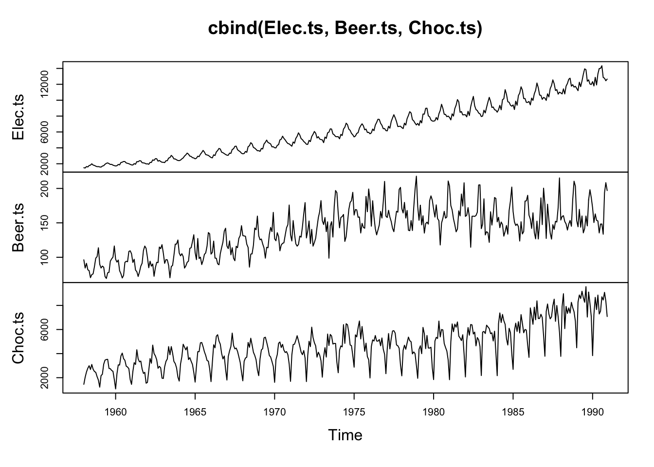
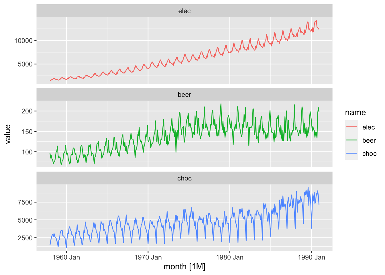
1.4.3 ‘electricity, beer, and chocolate’ Modern Look
Book code
<- read.table ("data/cbe.dat" , header = T)<- ts (CBE[, 3 ], start = 1958 , freq = 12 )<- ts (CBE[, 2 ], start = 1958 , freq = 12 )<- ts (CBE[, 1 ], start = 1958 , freq = 12 )plot (cbind (Elec.ts, Beer.ts, Choc.ts))
Tidyverts code
<- read_table ("data/cbe.dat" )<- lubridate:: ymd ("1958-01-01" )<- seq (start_date,+ months (nrow (cbe)- 1 ),by = "1 months" )<- cbe |> mutate (date = date_seq,month = tsibble:: yearmonth (date)) |> pivot_longer (choc: elec) |> mutate (name = factor (name,levels = c ("elec" , "beer" , "choc" ))) |> as_tsibble (index = month, key = name)autoplot (cbe_ts) + facet_wrap (~ name, ncol = 1 , scales = "free_y" )
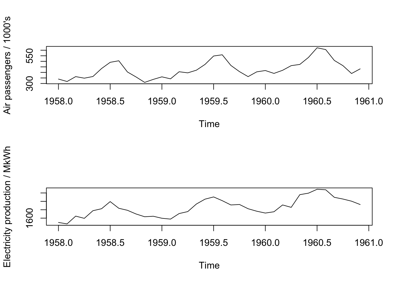
data (AirPassengers)<- AirPassengers<- ts.intersect (AP, Elec.ts)<- AP.elec[,1 ]<- AP.elec[,2 ]layout (1 : 2 )plot (AP, main = "" , ylab = "Air passengers / 1000's" )plot (Elec, main = "" , ylab = "Electricity production / MkWh" )
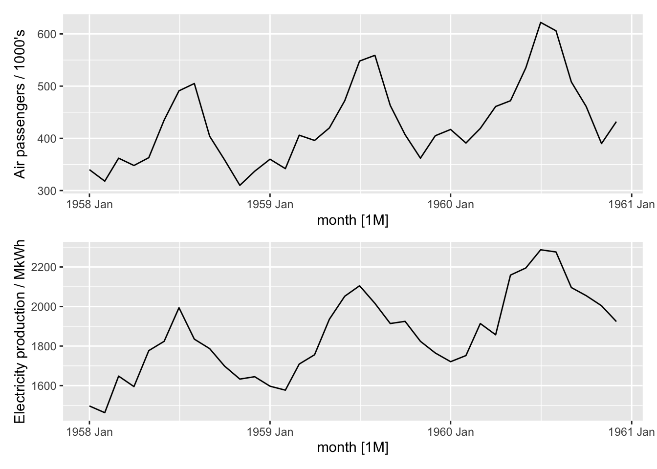
data (AirPassengers)<- as_tsibble (AirPassengers) |> mutate (Year = year (index),Month = month (index)<- cbe_ts |> rename (elec = value) |> filter (name == "elec" ) |> inner_join (rename (ap, airp = value),by = join_by (month == index)) <- autoplot (ap_elec, .vars = airp) + labs (y = "Air passengers / 1000's" )<- autoplot (ap_elec, .vars = elec) + labs (y = "Electricity production / MkWh" )/ ep
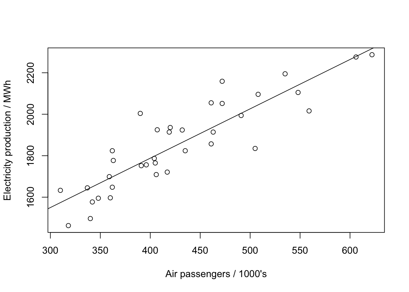
plot (as.vector (AP), as.vector (Elec),xlab = "Air passengers / 1000's" ,ylab = "Electricity production / MWh" )abline (reg = lm (Elec ~ AP))
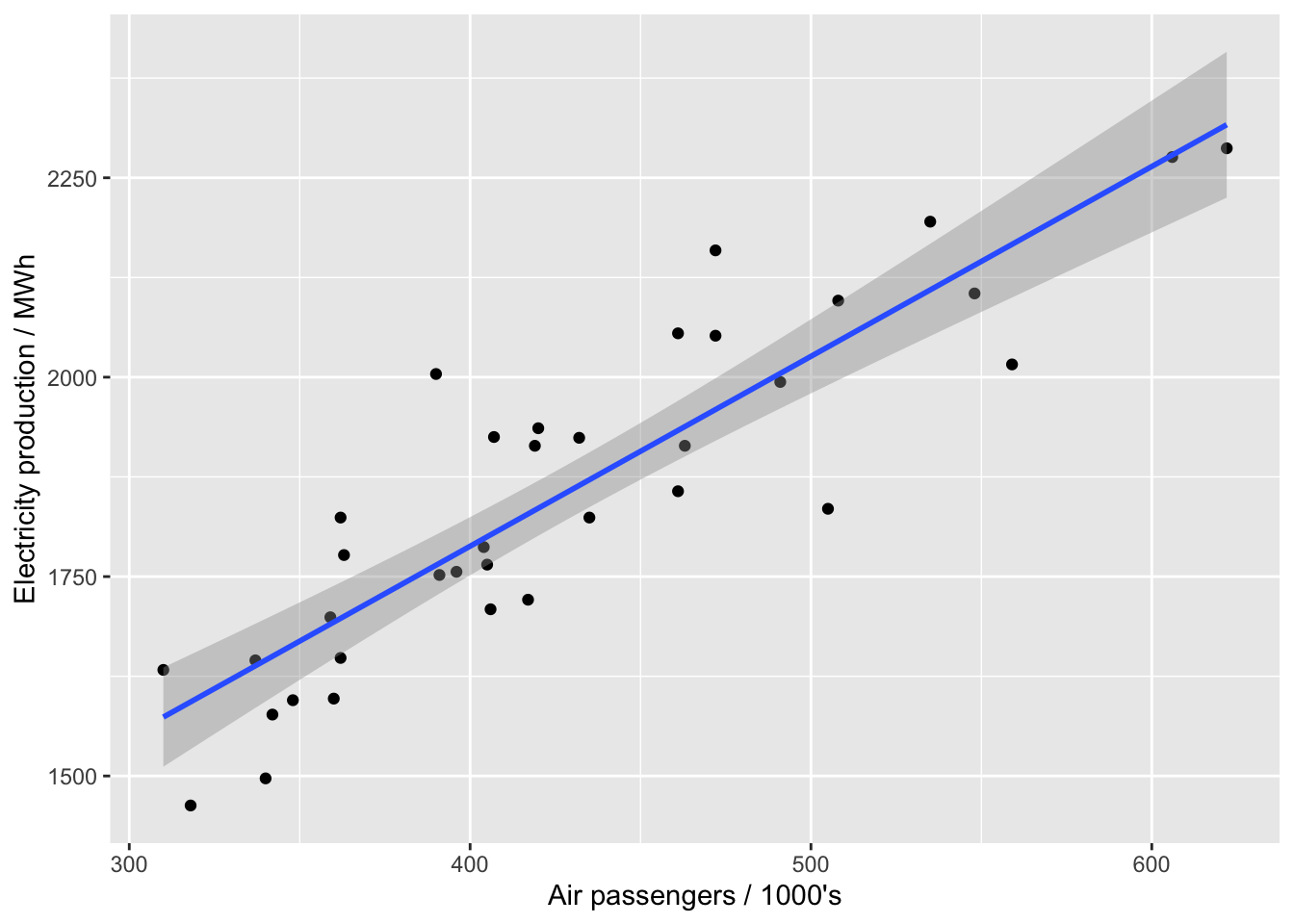
|> ggplot (aes (x = airp, y = elec)) + geom_point () + geom_smooth (method = "lm" ) + labs (x = "Air passengers / 1000's" ,y = "Electricity production / MWh"
cor (pull (ap_elec, airp), pull (ap_elec, elec))
Show the Book code in full
<- read.table ("data/cbe.dat" , header = T)<- ts (CBE[, 3 ], start = 1958 , freq = 12 )<- ts (CBE[, 2 ], start = 1958 , freq = 12 )<- ts (CBE[, 1 ], start = 1958 , freq = 12 )plot (cbind (Elec.ts, Beer.ts, Choc.ts))data (AirPassengers)<- AirPassengers<- ts.intersect (AP, Elec.ts)<- AP.elec[,1 ]<- AP.elec[,2 ]layout (1 : 2 )plot (AP, main = "" , ylab = "Air passengers / 1000's" )plot (Elec, main = "" , ylab = "Electricity production / MkWh" )plot (as.vector (AP), as.vector (Elec),xlab = "Air passengers / 1000's" ,ylab = "Electricity production / MWh" )abline (reg = lm (Elec ~ AP))cor (AP, Elec)
Show the Tidyverts code in full
<- read_table ("data/cbe.dat" )<- lubridate:: ymd ("1958-01-01" )<- seq (start_date,+ months (nrow (cbe)- 1 ),by = "1 months" )<- cbe |> mutate (date = date_seq,month = tsibble:: yearmonth (date)) |> pivot_longer (choc: elec) |> mutate (name = factor (name,levels = c ("elec" , "beer" , "choc" ))) |> as_tsibble (index = month, key = name)autoplot (cbe_ts) + facet_wrap (~ name, ncol = 1 , scales = "free_y" )data (AirPassengers)<- as_tsibble (AirPassengers) |> mutate (Year = year (index),Month = month (index)<- cbe_ts |> rename (elec = value) |> filter (name == "elec" ) |> inner_join (rename (ap, airp = value),by = join_by (month == index)) <- autoplot (ap_elec, .vars = airp) + labs (y = "Air passengers / 1000's" )<- autoplot (ap_elec, .vars = elec) + labs (y = "Electricity production / MkWh" )/ ep|> ggplot (aes (x = airp, y = elec)) + geom_point () + geom_smooth (method = "lm" ) + labs (x = "Air passengers / 1000's" ,y = "Electricity production / MWh" cor (pull (ap_elec, airp), pull (ap_elec, elec))
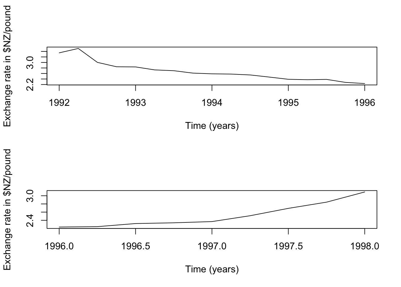
1.4.4 ‘Quarterly exchnage rate’ Modern Look
Book code
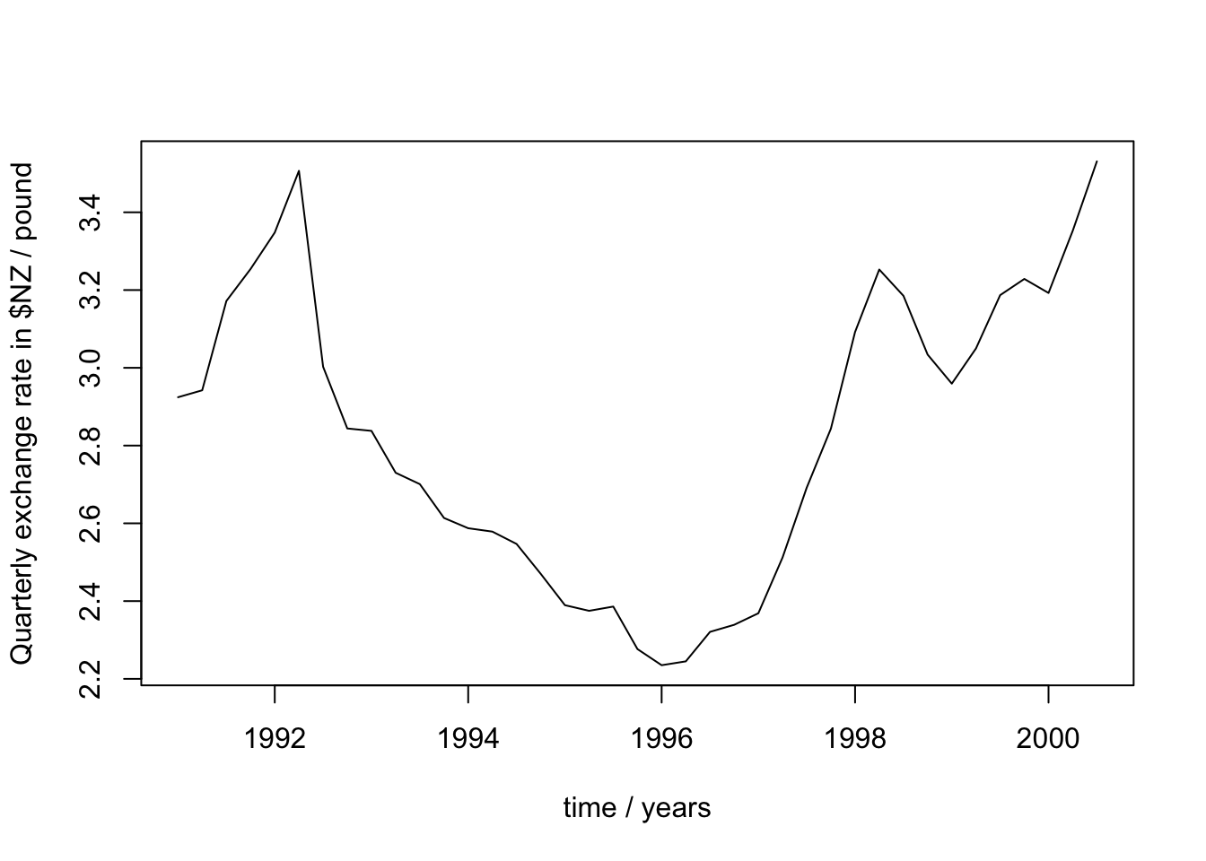
<- read.table ("data/pounds_nz.dat" , header = T)<- ts (Z, st = 1991 , fr = 4 )plot (Z.ts,xlab = "time / years" ,ylab = "Quarterly exchange rate in $NZ / pound" )
Tidyverts code
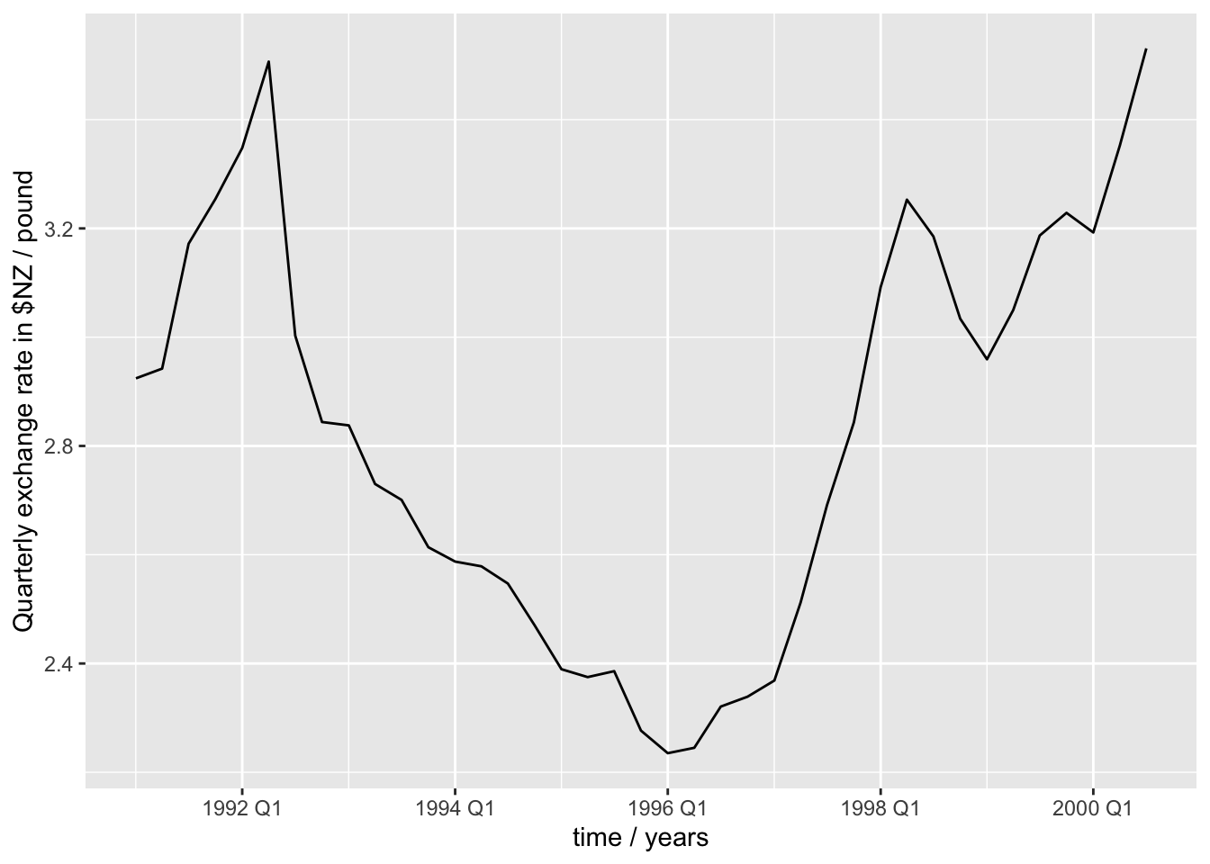
<- read_table ("data/pounds_nz.dat" )<- seq (:: ymd ("1991-01-01" ),by = "3 months" ,length.out = nrow (z))<- z |> mutate (date = date_seq,quarter = tsibble:: yearquarter (date)) |> as_tsibble (index = quarter)autoplot (z_ts) + labs (x = "time / years" ,y = "Quarterly exchange rate in $NZ / pound"
92.96 <- window (Z.ts, start = c (1992 , 1 ), end = c (1996 , 1 ))96.98 <- window (Z.ts, start = c (1996 , 1 ), end = c (1998 , 1 ))layout (1 : 2 )plot (Z.92.96 ,ylab = "Exchange rate in $NZ/pound" ,xlab = "Time (years)" )plot (Z.96.98 ,ylab = "Exchange rate in $NZ/pound" ,xlab = "Time (years)" )
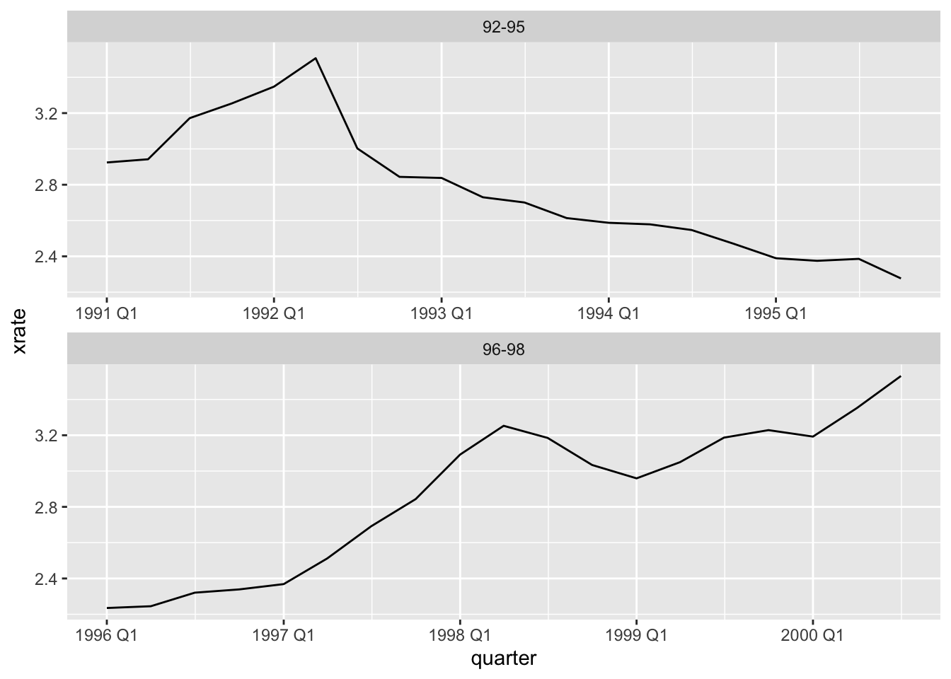
|> mutate (interval = ifelse (< ymd ("1996/01/01" ),"92-95" ,"96-98" )) |> ggplot (aes (x = quarter, y = xrate)) + geom_line () + facet_wrap (~ interval, ncol = 1 ,scales = "free_x" )
Show the Book code in full
<- read.table ("data/pounds_nz.dat" , header = T)<- ts (Z, st = 1991 , fr = 4 )plot (Z.ts,xlab = "time / years" ,ylab = "Quarterly exchange rate in $NZ / pound" )92.96 <- window (Z.ts, start = c (1992 , 1 ), end = c (1996 , 1 ))96.98 <- window (Z.ts, start = c (1996 , 1 ), end = c (1998 , 1 ))layout (1 : 2 )plot (Z.92.96 ,ylab = "Exchange rate in $NZ/pound" ,xlab = "Time (years)" )plot (Z.96.98 ,ylab = "Exchange rate in $NZ/pound" ,xlab = "Time (years)" )
Show the Tidyverts code in full
<- read_table ("data/pounds_nz.dat" )<- seq (:: ymd ("1991-01-01" ),by = "3 months" ,length.out = nrow (z))<- z |> mutate (date = date_seq,quarter = tsibble:: yearquarter (date)) |> as_tsibble (index = quarter)autoplot (z_ts) + labs (x = "time / years" ,y = "Quarterly exchange rate in $NZ / pound" |> mutate (interval = ifelse (< ymd ("1996/01/01" ),"92-95" ,"96-98" )) |> ggplot (aes (x = quarter, y = xrate)) + geom_line () + facet_wrap (~ interval, ncol = 1 ,scales = "free_x" )
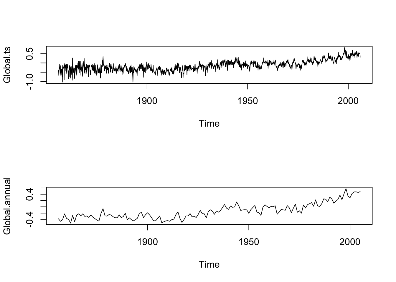
1.4.5 ‘Global temperature series’ Modern Look
Book code
<- scan ("data/global.dat" )<- ts (Global,st = c (1856 , 1 ),end = c (2005 , 12 ),fr = 12 )<- aggregate (Global.ts, FUN = mean)layout (1 : 2 )plot (Global.ts)plot (Global.annual)
Tidyverts code
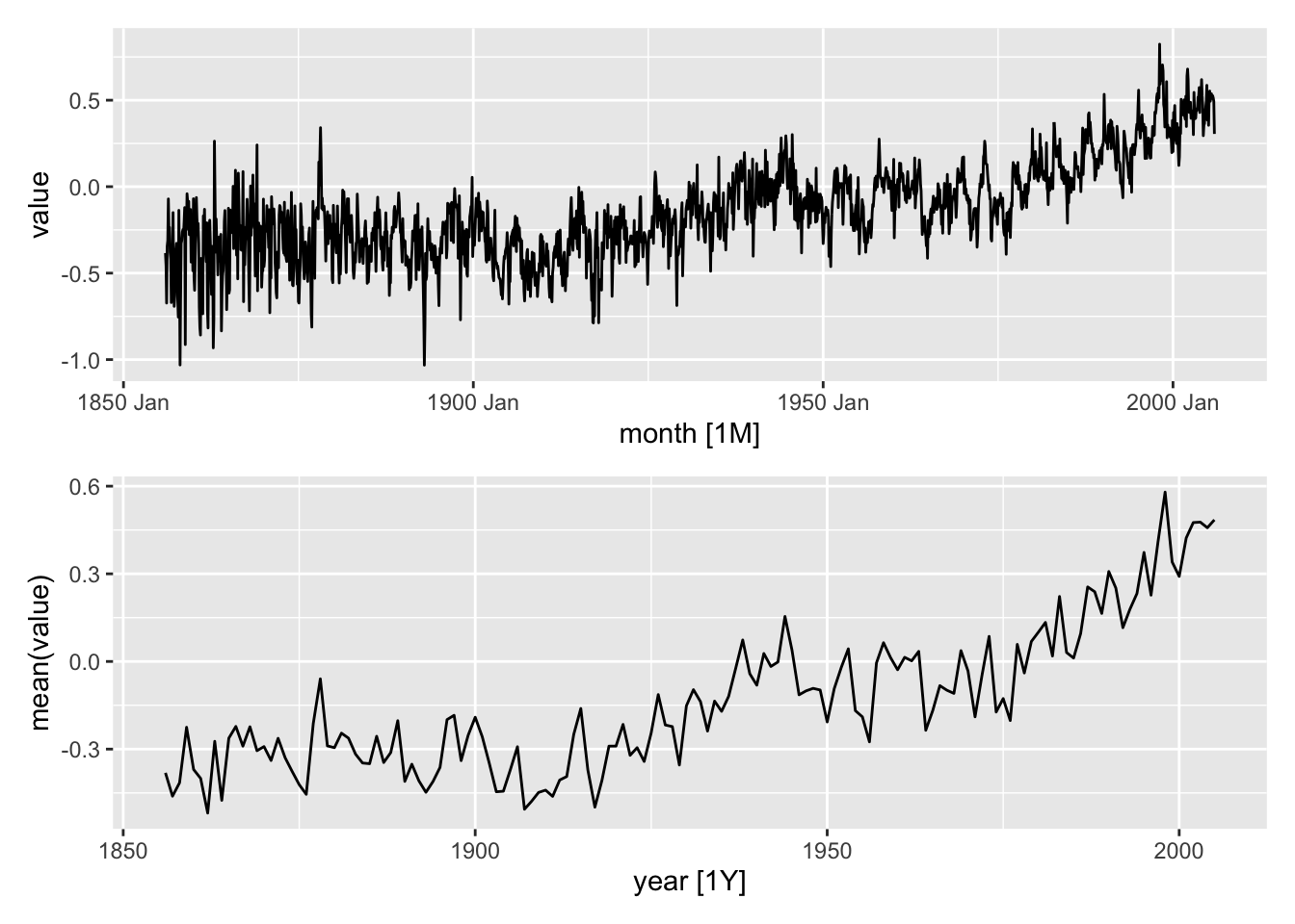
<- scan ("data/global.dat" )<- seq (:: ymd ("1856-01-01" ),by = "1 months" ,length.out = length (global))<- tibble (date = date_seq,value = global,month = tsibble:: yearmonth (date_seq),year = lubridate:: year (date_seq))<- as_tsibble (global_df, index = month)<- global_df |> summarise (mean (value), .by = year) |> as_tsibble (index = year)<- autoplot (global_ts)<- autoplot (global_annual_ts)/ ga
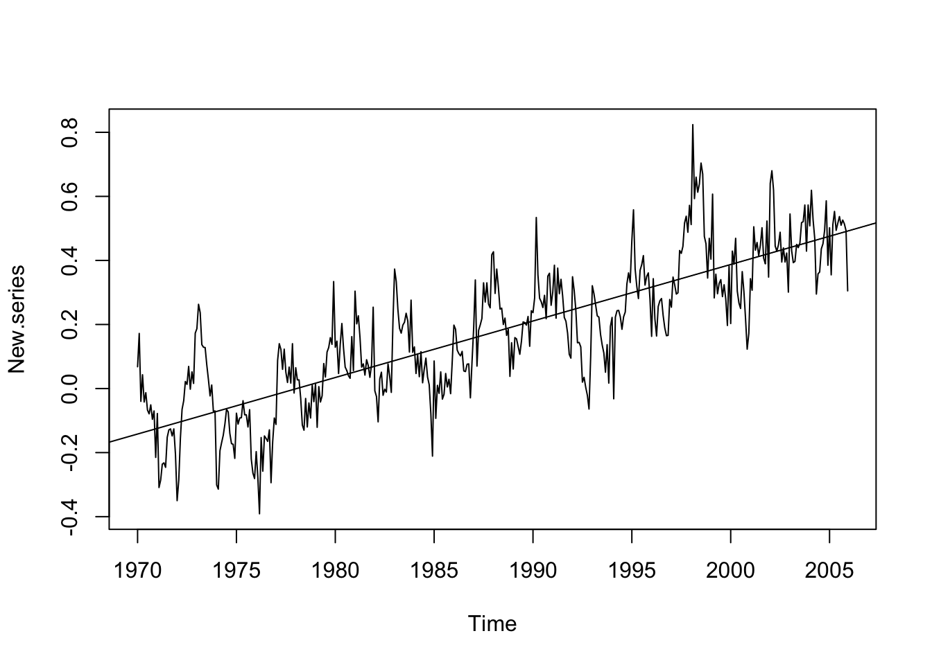
<- window (Global.ts, start= c (1970 , 1 ), end= c (2005 , 12 ))<- time (New.series)plot (New.series); abline (reg= lm (New.series ~ New.time))
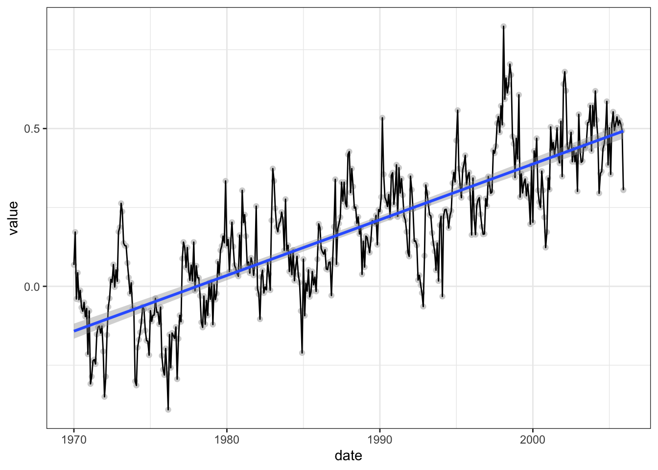
|> filter (date >= ymd ("1970-01-01" ), date <= ymd ("2005-12-31" )) |> ggplot (aes (x = date, y = value)) + geom_point (color = "lightgrey" ) + geom_line () + geom_smooth (method = "lm" ) + theme_bw ()
Show the Book code in full
<- scan ("data/global.dat" )<- ts (Global,st = c (1856 , 1 ),end = c (2005 , 12 ),fr = 12 )<- aggregate (Global.ts, FUN = mean)plot (Global.ts)plot (Global.annual)<- window (Global.ts, start= c (1970 , 1 ), end= c (2005 , 12 ))<- time (New.series)plot (New.series); abline (reg= lm (New.series ~ New.time))
Show the Tidyverts code in full
<- scan ("data/global.dat" )<- seq (:: ymd ("1856-01-01" ),by = "1 months" ,length.out = length (global))<- tibble (date = date_seq,value = global,month = tsibble:: yearmonth (date_seq),year = lubridate:: year (date_seq))<- as_tsibble (global_df, index = month)<- global_df |> summarise (mean (value), .by = year) |> as_tsibble (index = year)<- autoplot (global_ts)<- autoplot (global_annual_ts)/ ga|> filter (date >= ymd ("1970-01-01" ), date <= ymd ("2005-12-31" )) |> ggplot (aes (x = date, y = value)) + geom_point (color = "lightgrey" ) + geom_line () + geom_smooth (method = "lm" ) + theme_bw ()
1.5.5 ‘Decomposition in R’ Modern Look
Tidyverts code
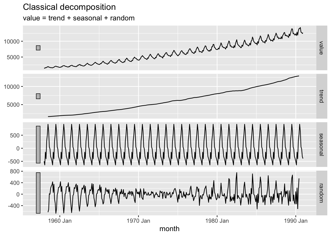
<- filter (cbe_ts, name == "elec" ) |> model (feasts:: classical_decomposition (value,type = "add" )) |> components ()autoplot (elec_decompose)
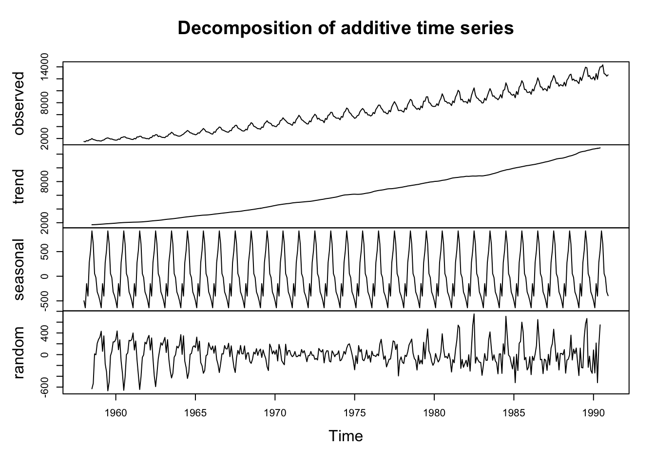
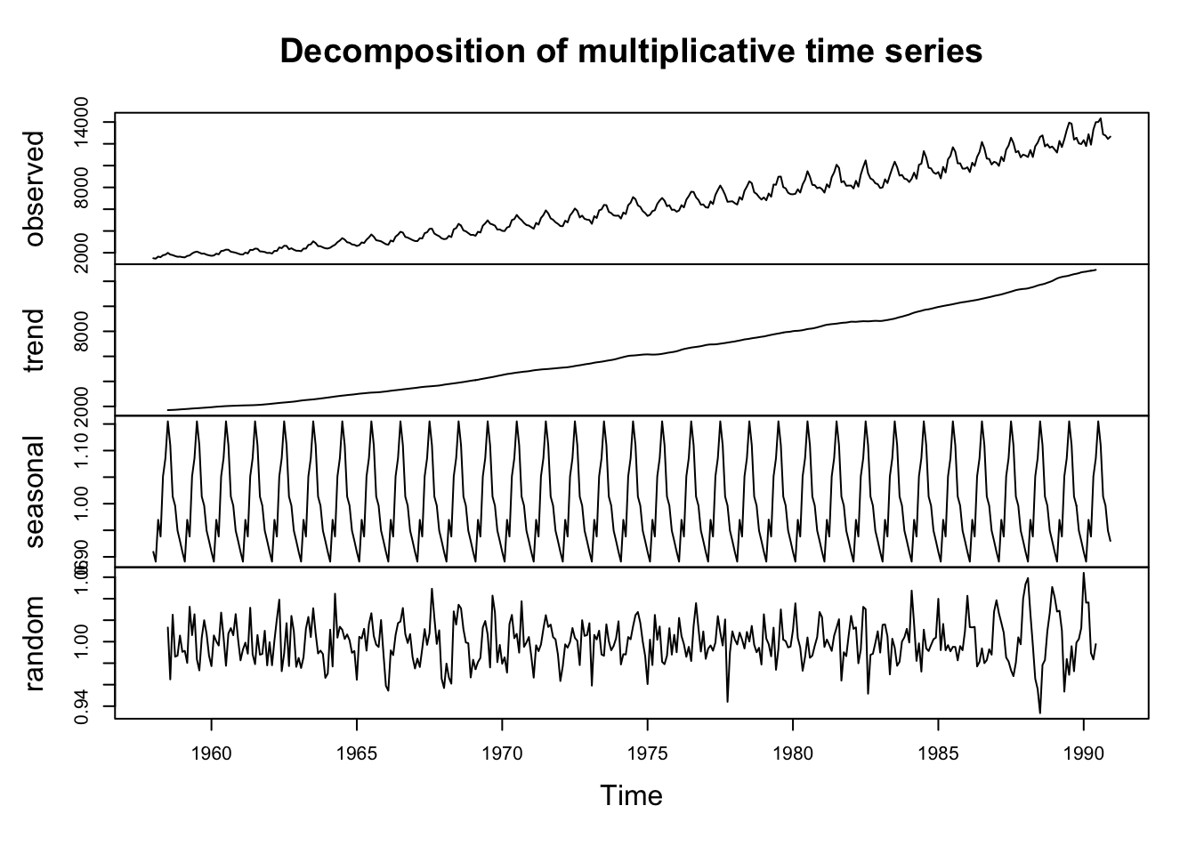
<- decompose (Elec.ts, type = "mult" )plot (Elec.decom)
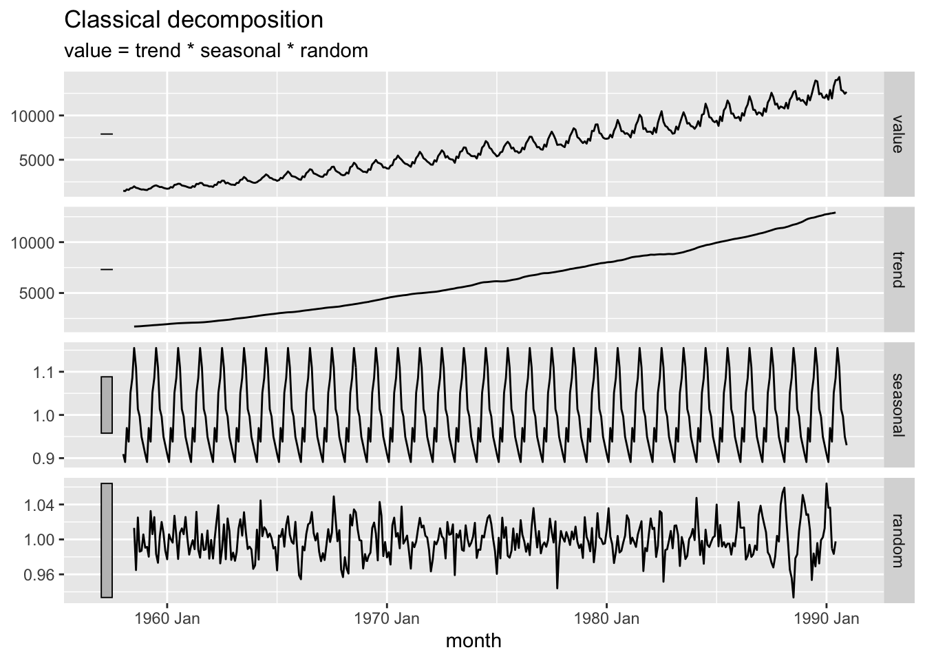
<- filter (cbe_ts, name == "elec" ) |> model (feasts:: classical_decomposition (value,type = "mult" )) |> components ()autoplot (elec_decompose)
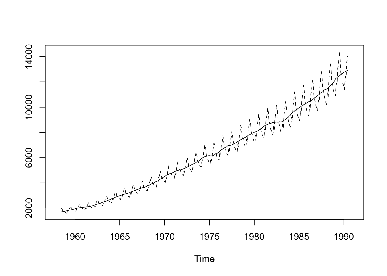
<- Elec.decom$ trend<- Elec.decom$ seasonalts.plot (cbind (Trend, Trend * Seasonal), lty = 1 : 2 )
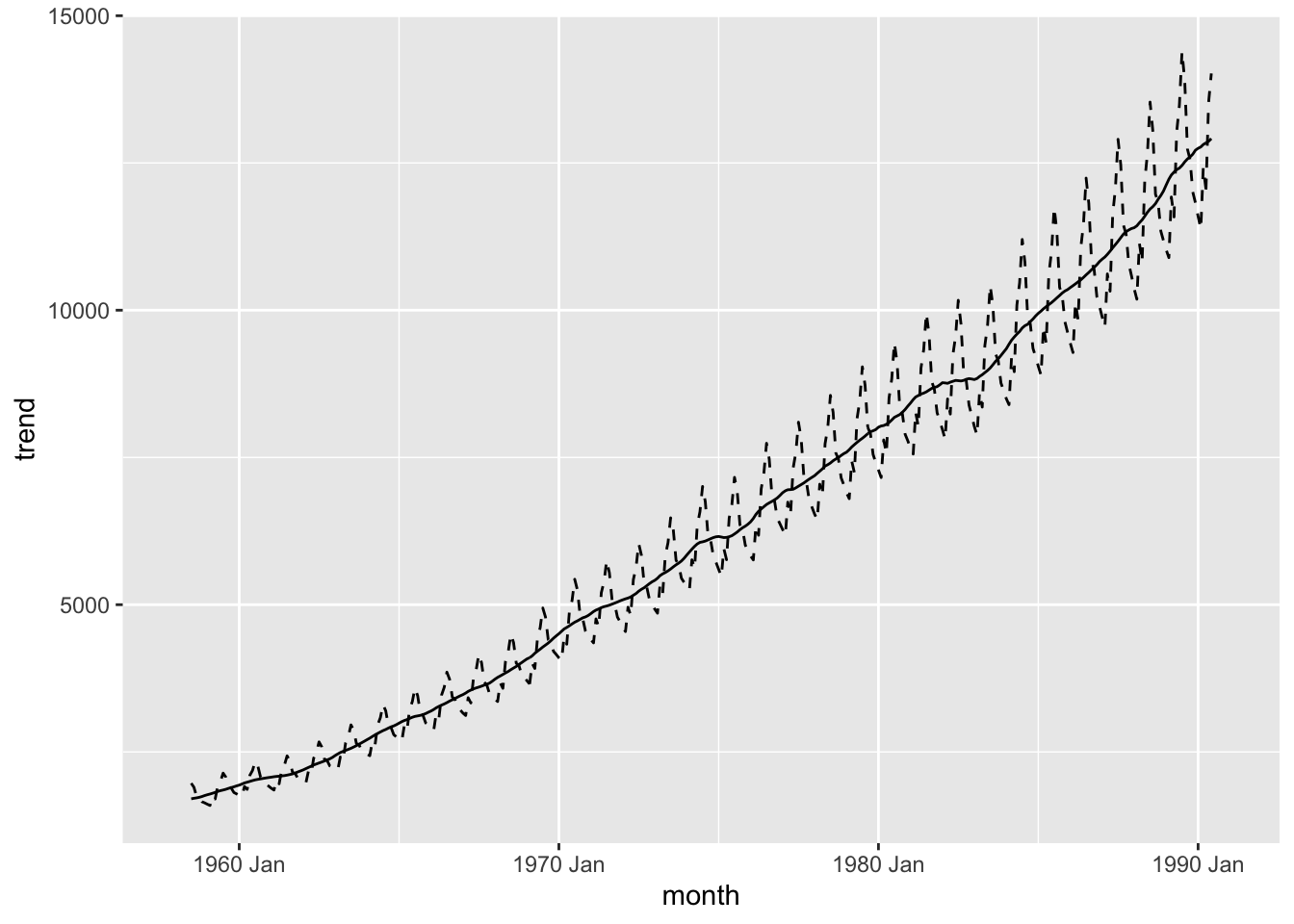
|> ggplot (aes (x = month)) + geom_line (aes (y = trend)) + geom_line (aes (y = trend * seasonal), linetype = 2 )
Show the Book code in full
plot (decompose (Elec.ts))<- decompose (Elec.ts, type = "mult" )plot (Elec.decom)<- Elec.decom$ trend<- Elec.decom$ seasonalts.plot (cbind (Trend, Trend * Seasonal), lty = 1 : 2 )
Show the Tidyverts code in full
<- filter (cbe_ts, name == "elec" ) |> model (feasts:: classical_decomposition (value,type = "add" )) |> components ()autoplot (elec_decompose)<- filter (cbe_ts, name == "elec" ) |> model (feasts:: classical_decomposition (value,type = "mult" )) |> components ()autoplot (elec_decompose)|> ggplot (aes (x = month)) + geom_line (aes (y = trend)) + geom_line (aes (y = trend * seasonal), linetype = 2 )
1.6 Summary of modern R commands used in examples