set.seed(1)
w <- rnorm(100)
plot(w, type = "l")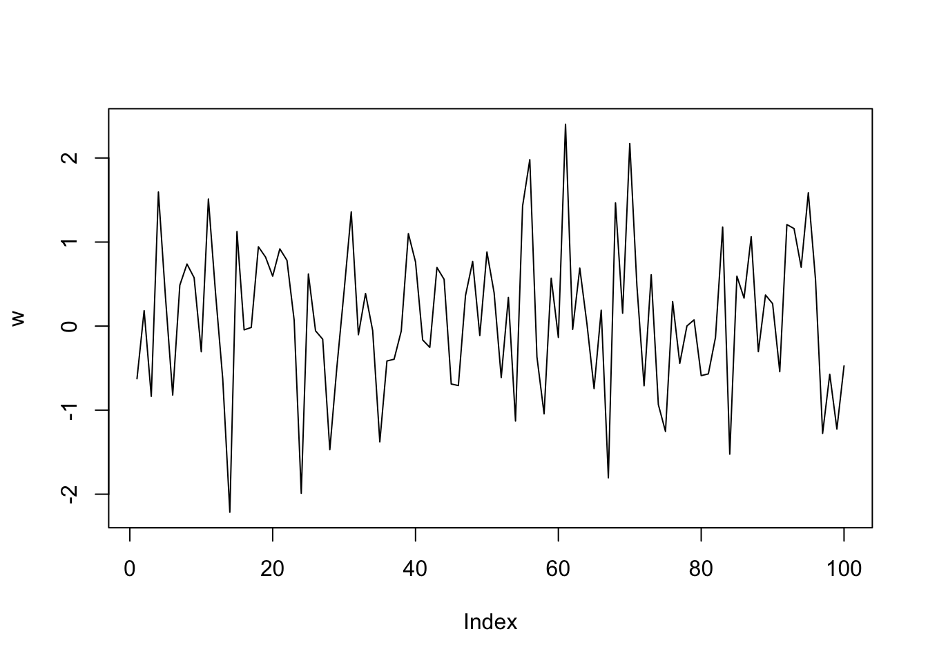
Throughout this book, we will often fit models to data that we have simulated and attempt to recover the underlying model parameters. At first sight, this might seem odd, given that the parameters are used to simulate the data so that we already know at the outset the values the parameters should take. However, the procedure is useful for a number of reasons. In particular, to be able to simulate data using a model requires that the model formulation be correctly understood. If the model is understood but incorrectly implemented, then the parameter estimates from the fitted model may deviate significantly from the underlying model values used in the simulation. Simulation can therefore help ensure that the model is both correctly understood and correctly implemented.
R” Modern LookBook code
set.seed(1)
w <- rnorm(100)
plot(w, type = "l")
Tidyverts code
pacman::p_load("tsibble", "fable", "feasts",
    "tsibbledata", "fable.prophet", "tidyverse", "patchwork")
set.seed(1)
wd <- tibble(
    x = 1:100,
    y = rnorm(100))
wd |> ggplot(aes(x = x, y = y)) + geom_line()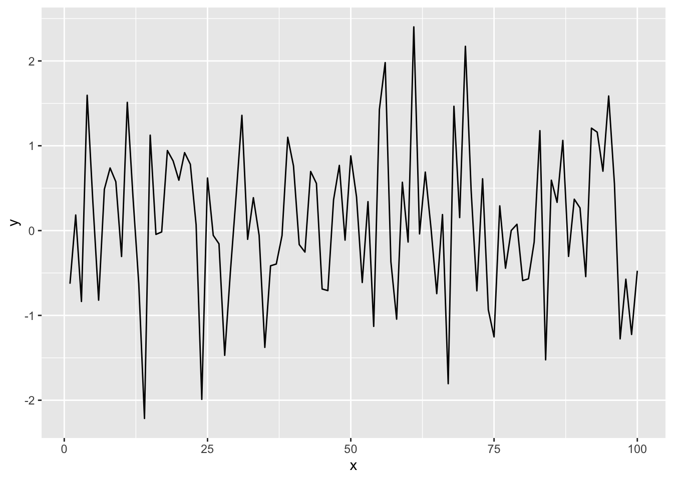
x <- seq(-3, 3, length = 1000)
hist(rnorm(100), prob = T)
points(x, dnorm(x), type = "l")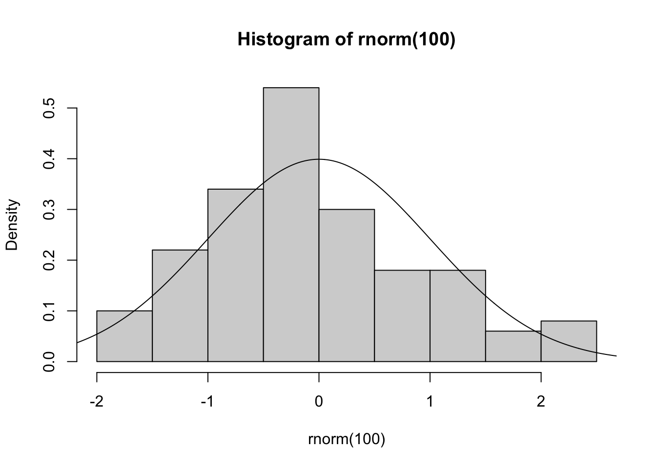
xd <- tibble(
    x = seq(-3, 3, length = 1000),
    norm = rnorm(1000),
    density = dnorm(x)
)
xd |>
    ggplot(aes(x = norm)) +
    geom_histogram(aes(y = after_stat(density)),
        color = "white", fill = "darkgrey") +
    geom_line(aes(x = x, y = density)) +
    theme_bw()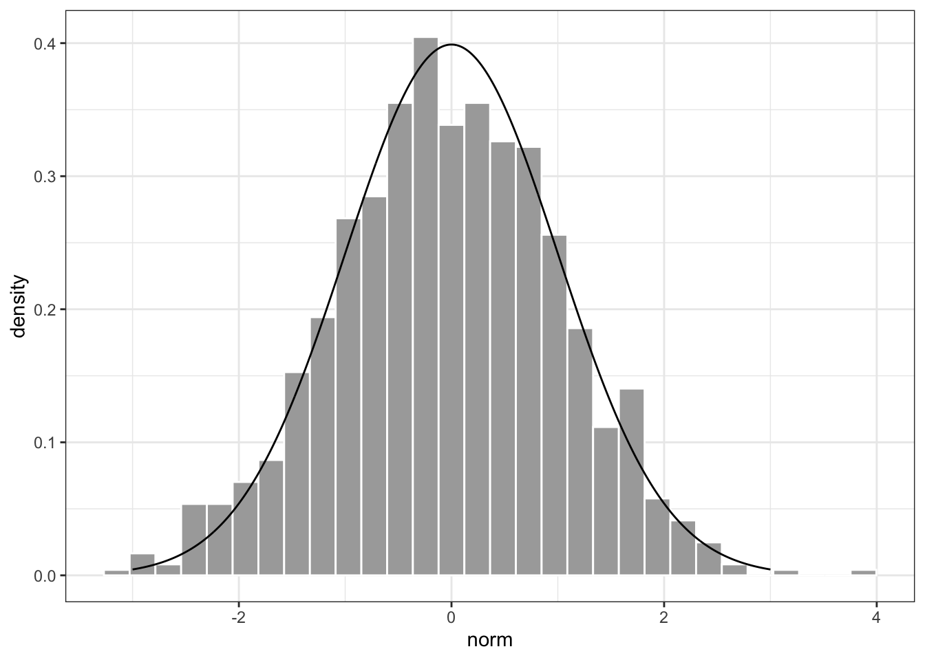
set.seed(1)
wd <- tibble(
    x = 1:100,
    y = rnorm(100))
wd |> ggplot(aes(x = x, y = y)) + geom_line()
xd <- tibble(
    x = seq(-3, 3, length = 1000),
    norm = rnorm(1000),
    density = dnorm(x)
)
xd |>
    ggplot(aes(x = norm)) +
    geom_histogram(aes(y = after_stat(density)),
        color = "white", fill = "darkgrey") +
    geom_line(aes(x = x, y = density)) +
theme_bw()Book code
set.seed(2)
acf(rnorm(100))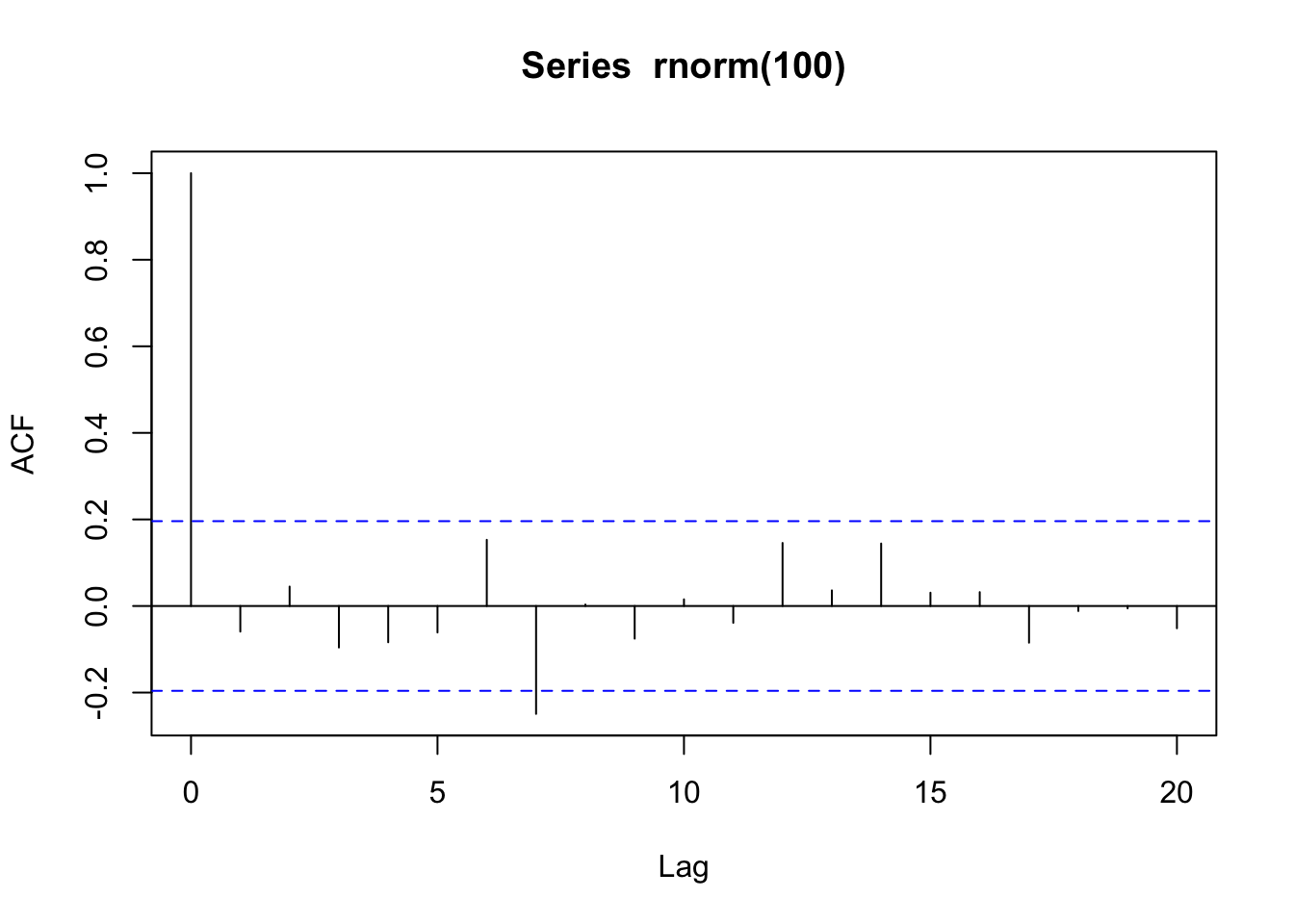
Tidyverts code
set.seed(2)
tsibble(seq = 1:100,
        values = rnorm(100),
        index = seq) |>
    ACF(values) |>
    autoplot()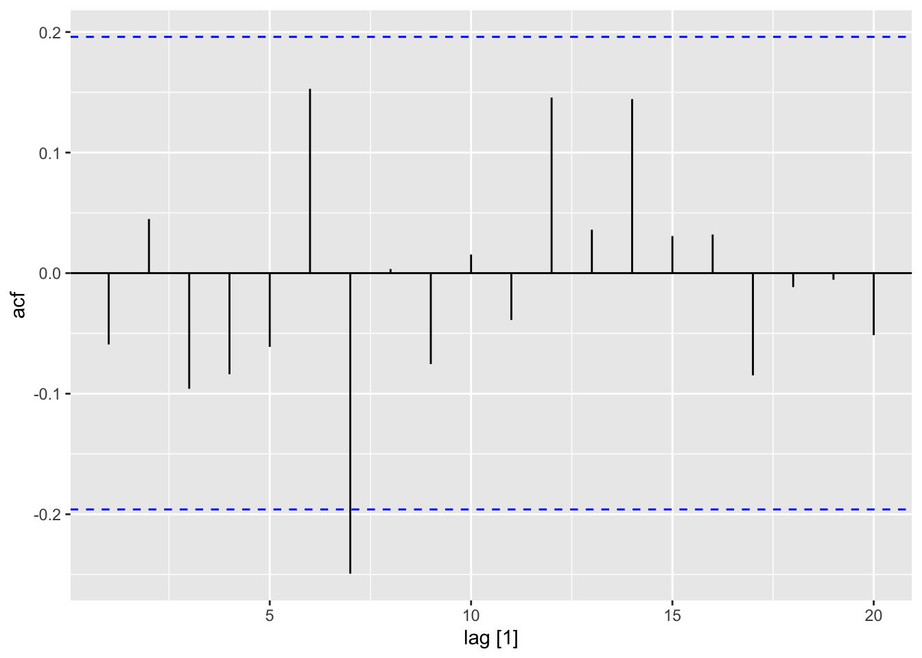
Book code
set.seed(2)
x <- w <- rnorm(1000)
for (t in 2:1000) x[t] <- x[t - 1] + w[t]
plot(x, type = "l")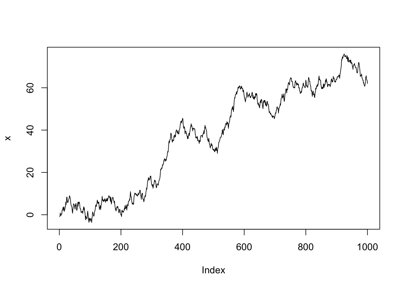
Tidyverts code
set.seed(2)
dat <- tibble(w = rnorm(1000)) |>
    mutate(
        index = 1:n(),
         x = purrr::accumulate2(
            lag(w), w,
            \(acc, nxt, w) acc + w,
            .init = 0)[-1]) |>
    tsibble::as_tsibble(index = index)
autoplot(dat, .var = x)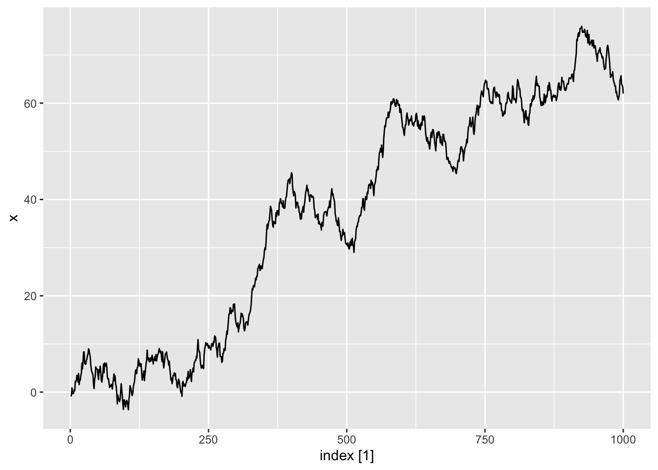
acf(x)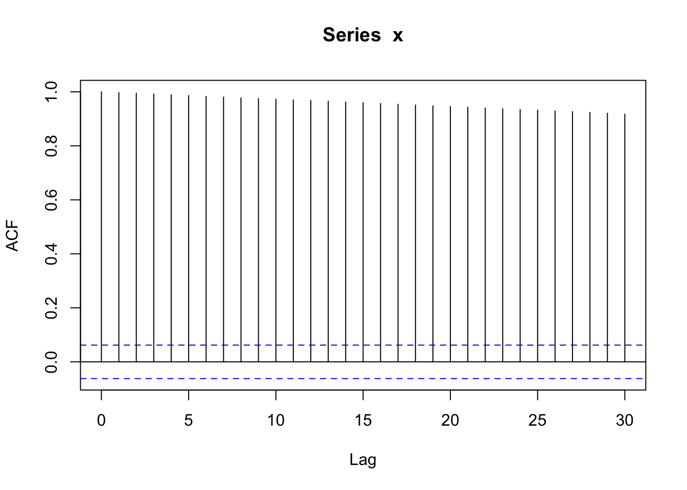
ACF(dat, x) |>
    autoplot()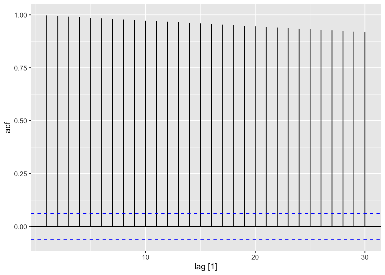
Book code
acf(diff(x))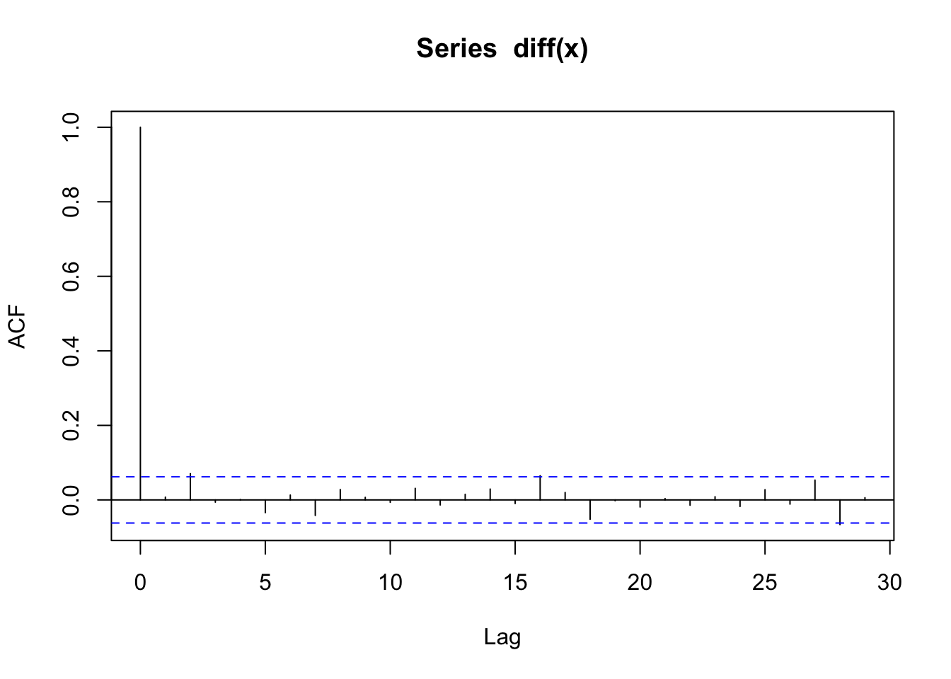
Tidyverts code
dat |>
    mutate(diff = x - lag(x)) |>
    ACF(diff) |>
    autoplot()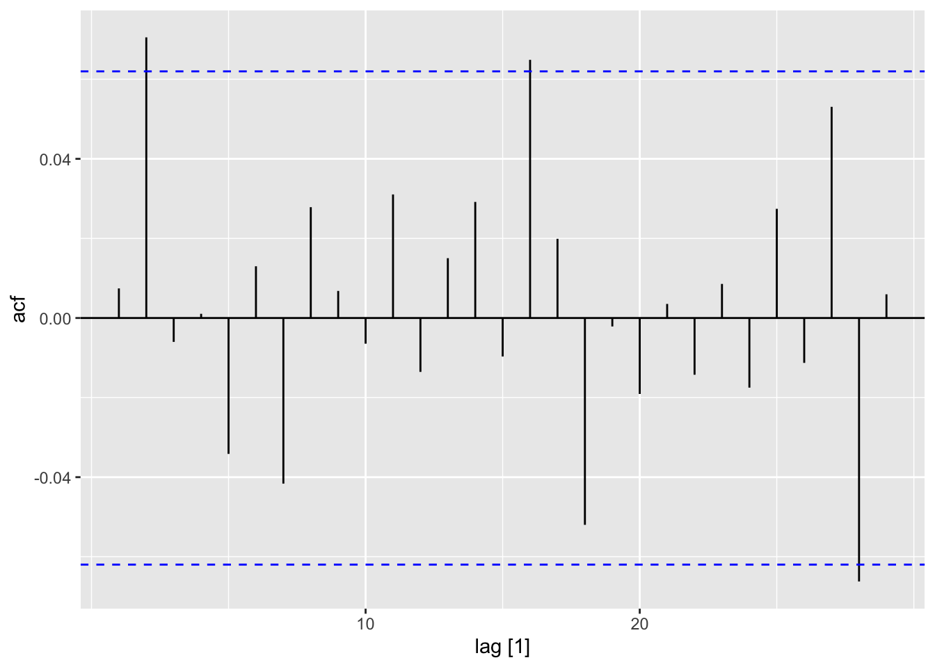
Book code
Z <- read.table("data/pounds_nz.dat", header = T)
Z.ts <- ts(Z, st = 1991, fr = 4)
acf(diff(Z.ts))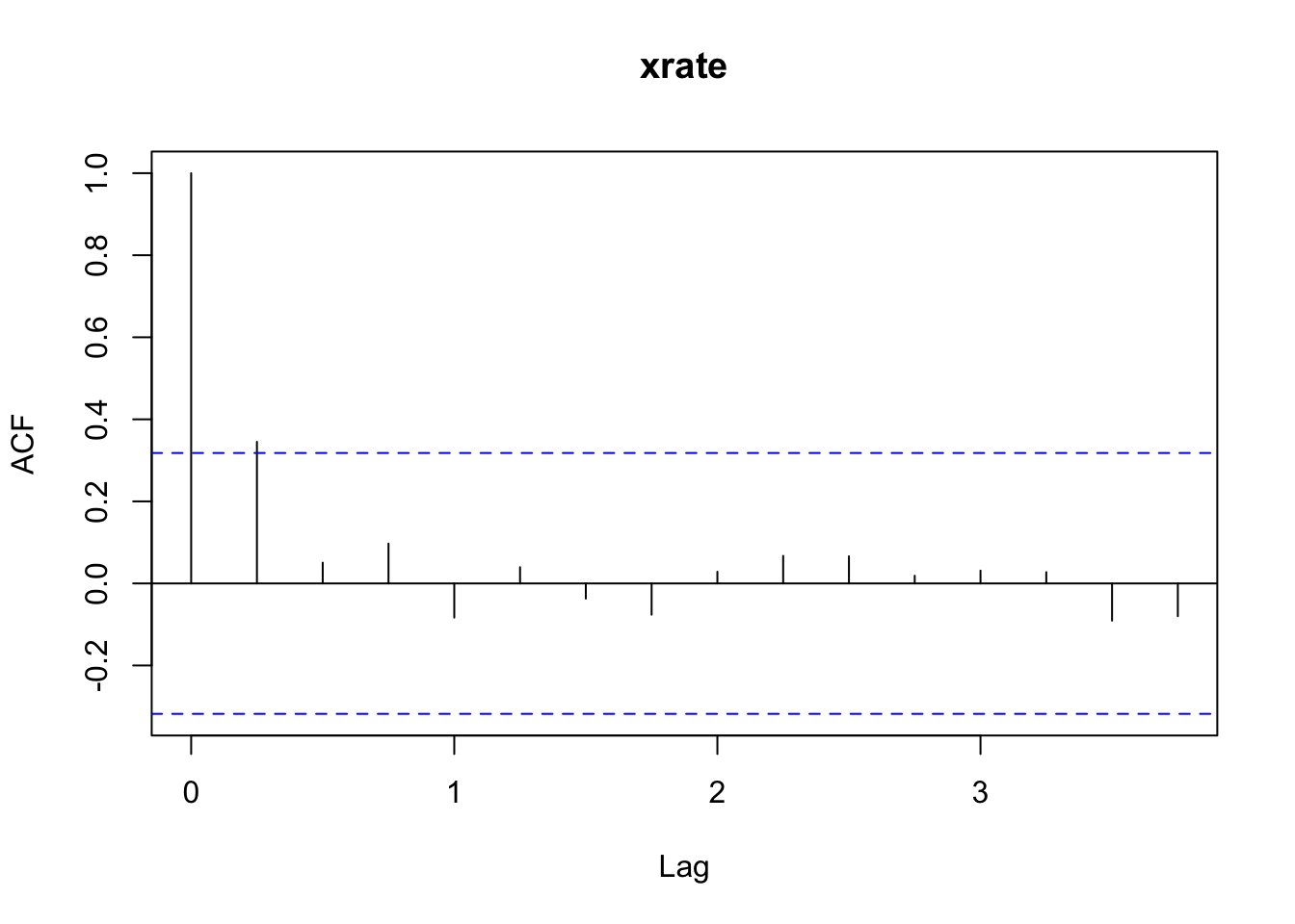
Tidyverts code
z <- read_table("data/pounds_nz.dat")
date_seq <- seq(
    lubridate::ymd("1991-01-01"),
    by = "3 months",
    length.out = nrow(z))
z_ts <- z |>
    mutate(
        date = date_seq,
        quarter = tsibble::yearquarter(date)) |>
    as_tsibble(index = quarter)
z_ts |>
    mutate(diff = xrate - lag(xrate)) |>
    ACF(diff) |>
    autoplot()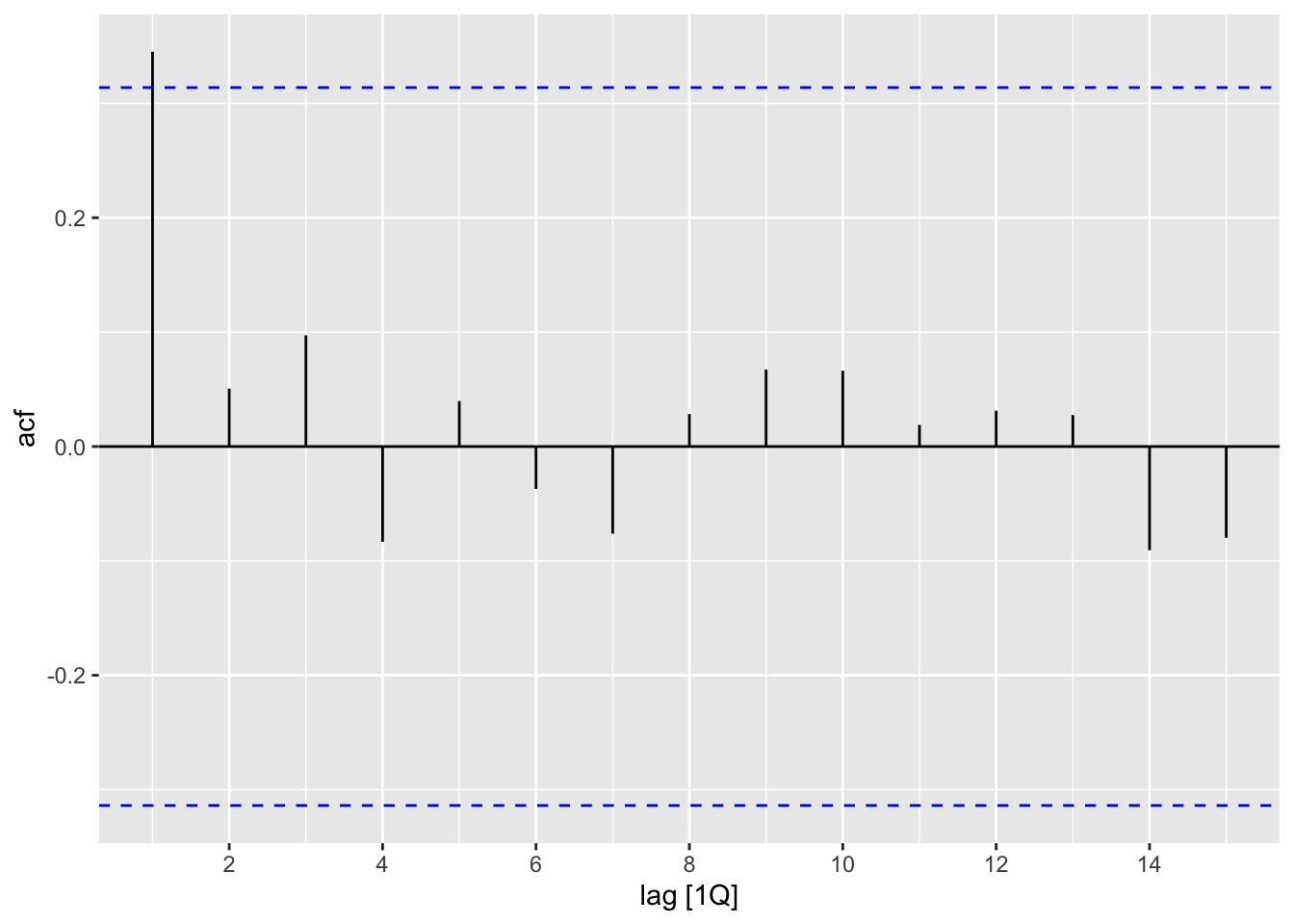
Z.hw <- HoltWinters(Z.ts, alpha = 1, gamma = FALSE) # changed from book
acf(resid(Z.hw)) # not exact match.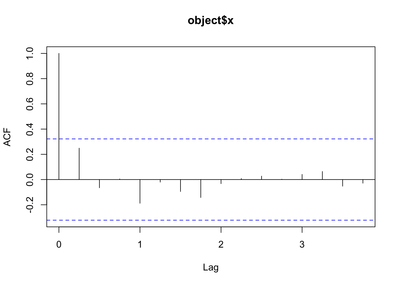
z_hw <- z_ts |>
    model(Additive = ETS(xrate ~
        trend("A", alpha = 1) +
        error("A") + season("N", gamma = 0),
        opt_crit = "amse", nmse = 1)) |>
        residuals()
ACF(z_hw, .resid) |>
    autoplot()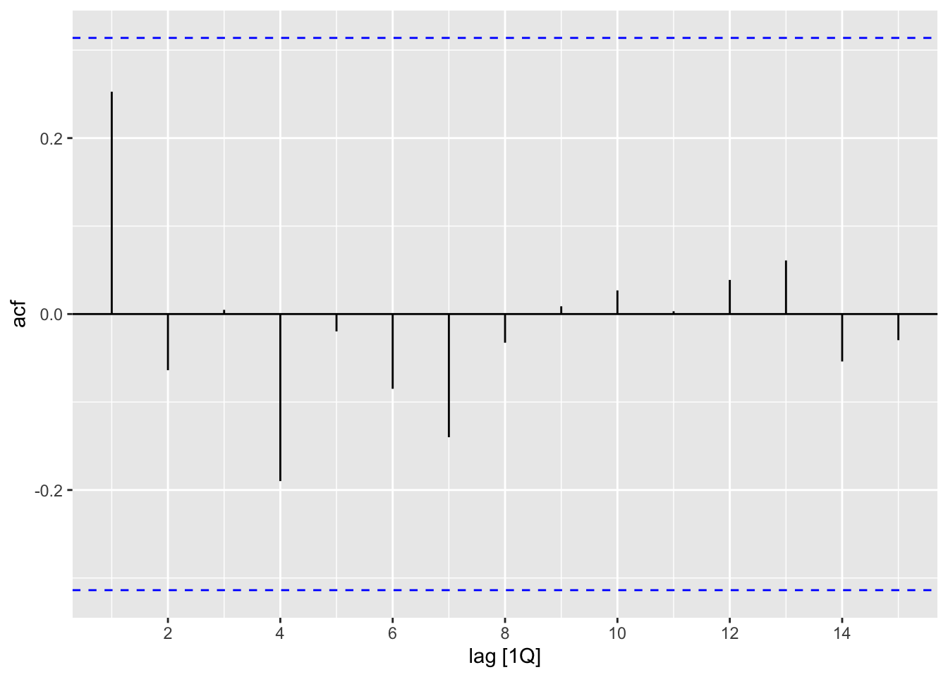
z <- read_table("data/pounds_nz.dat")
date_seq <- seq(
    lubridate::ymd("1991-01-01"),
    by = "3 months",
    length.out = nrow(z))
z_ts <- z |>
    mutate(
        date = date_seq,
        quarter = tsibble::yearquarter(date)) |>
    as_tsibble(index = quarter)
z_ts |>
    mutate(diff = xrate - lag(xrate)) |>
    ACF(diff) |>
    autoplot()
z_hw <- z_ts |>
    model(Additive = ETS(xrate ~
        trend("A", alpha = 1) +
        error("A") + season("N", gamma = 0),
        opt_crit = "amse", nmse = 1)) |>
        residuals()
ACF(z_hw, .resid) |>
autoplot()Book code
HP.dat <- read.table("data/HP.txt", header = T)
# attach(HP.dat) # bad practice
plot(as.ts(HP.dat$Price))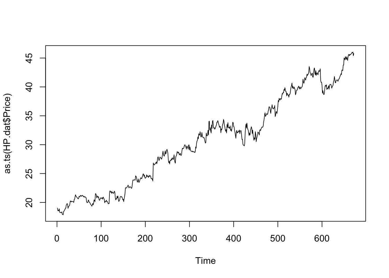
Tidyverts code
hp_dat <- read_table("data/HP.txt") |>
    mutate(Day = 1:n())
ggplot(hp_dat, aes(x = Day, y = Price)) + geom_line()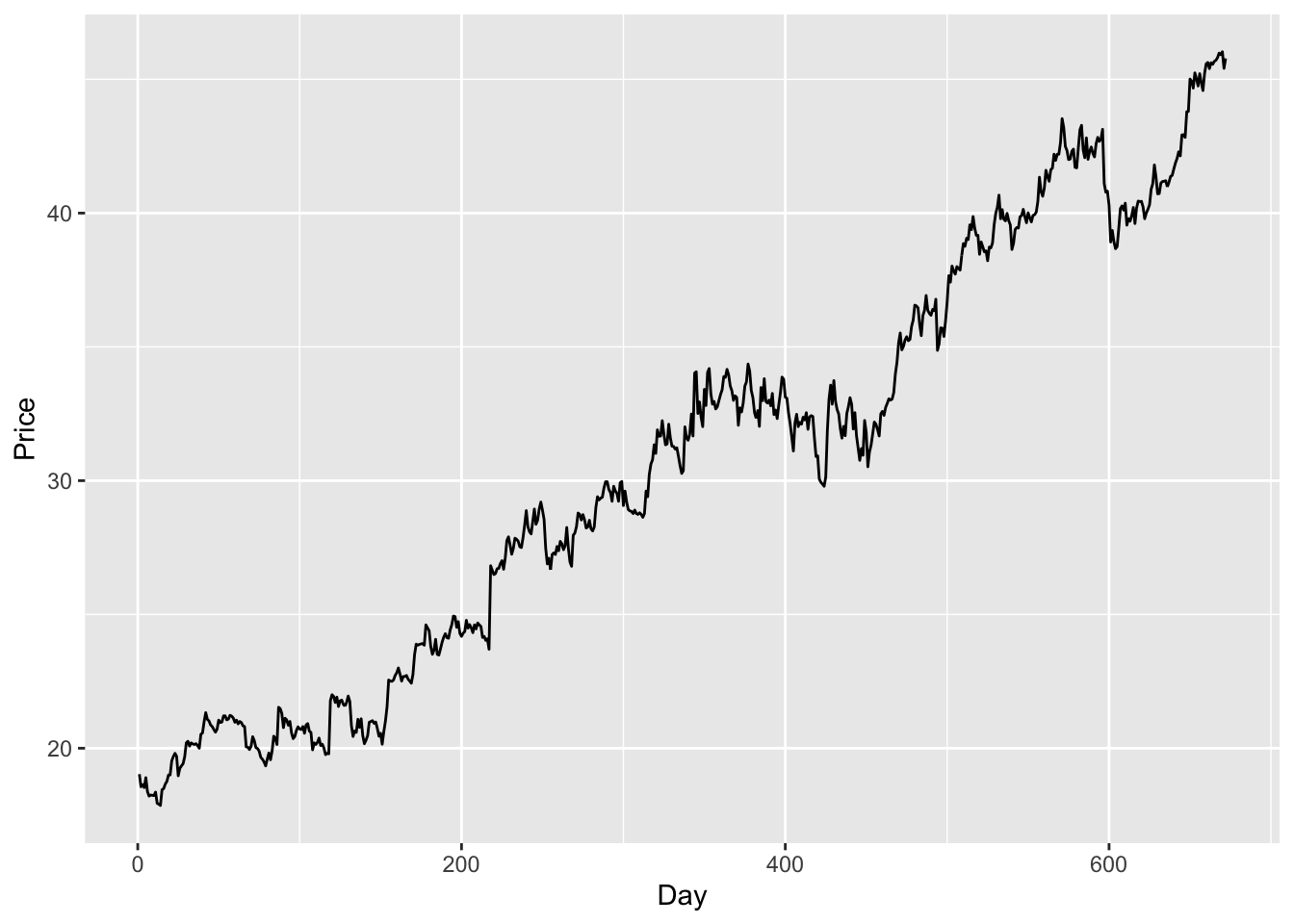
DP <- diff(HP.dat$Price)
plot(as.ts(DP))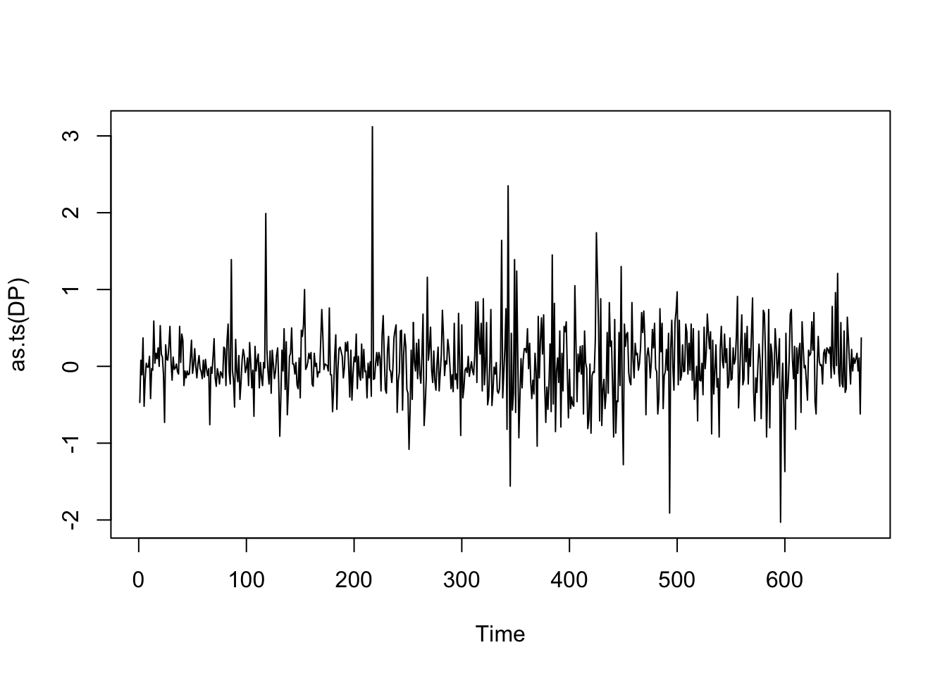
hp_dat |>
    mutate(diff = Price - lag(Price)) |>
ggplot(aes(x = Day, y = diff)) +
    geom_line()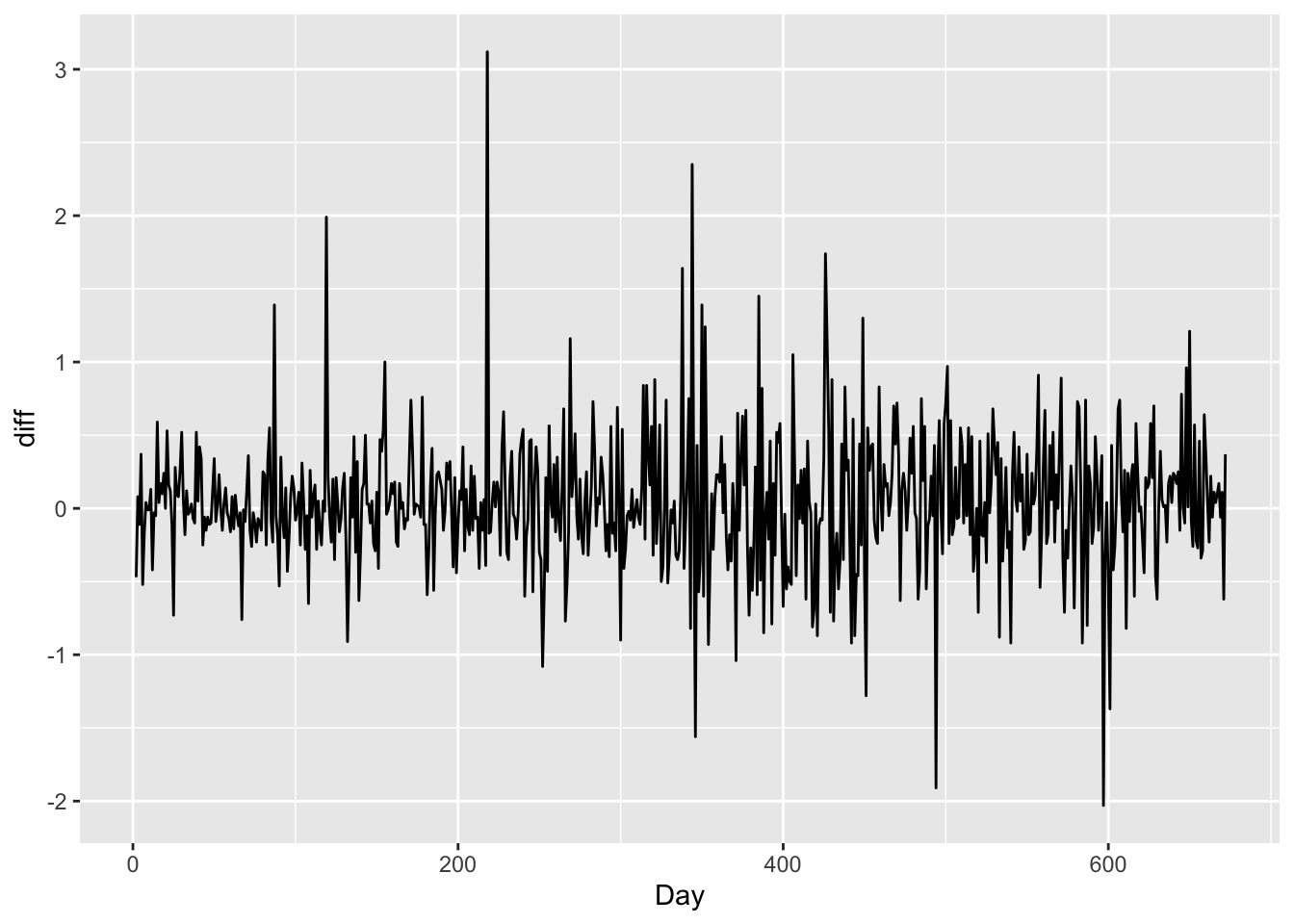
acf(DP)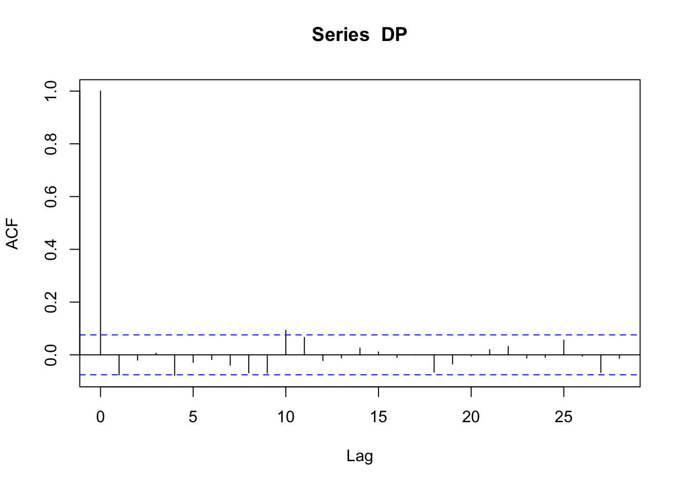
hp_dat |>
    mutate(diff = Price - lag(Price)) |>
    as_tsibble(index = Day) |>
ACF(diff) |>
    autoplot()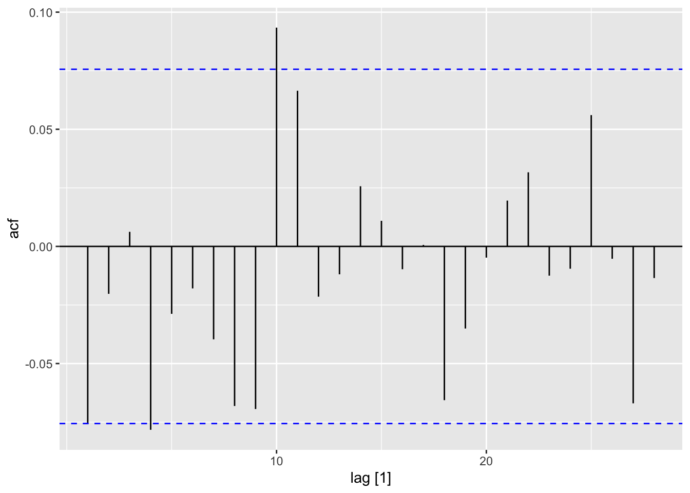
mean(DP) + c(-2, 2) * sd(DP) / sqrt(length(DP))[1] 0.004378275 0.075353468hp_dat |>
mutate(diff = Price - lag(Price)) |>
slice(-1) |>
summarize(
mean = mean(diff),
sd = sd(diff),
n = n(),
std_error = sd / sqrt(n),
lower = mean - 2 * std_error,
upper = mean + 2 * std_error)# A tibble: 1 × 6
mean sd n std_error lower upper
<dbl> <dbl> <int> <dbl> <dbl> <dbl>
1 0.0399 0.460 671 0.0177 0.00438 0.0754hp_dat <- read_table("data/HP.txt") |>
mutate(Day = 1:n())
ggplot(hp_dat, aes(x = Day, y = Price))
geom_line()
hp_dat |>
mutate(diff = Price - lag(Price)) |>
ggplot(aes(x = Day, y = diff)) +
geom_line()
hp_dat |>
mutate(diff = Price - lag(Price)) |>
as_tsibble(index = Day) |>
ACF(diff) |>
autoplot()
hp_dat |>
    mutate(diff = Price - lag(Price)) |>
    slice(-1) |>
    summarize(
        mean = mean(diff),
        sd = sd(diff),
        n = n(),
        std_error = sd / sqrt(n),
        lower = mean - 2 * std_error,
upper = mean + 2 * std_error)Book code
rho <- function(k, alpha) alpha^k
layout(1:2)
plot(0:10, rho(0:10, 0.7), type = "b")
plot(0:10, rho(0:10, -0.7), type = "b")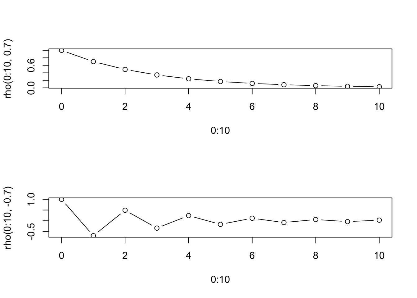
Tidyverts code
rho <- function(k, alpha) alpha^k
dat <- tibble(
        x = 0:10,
        a7 = rho(x, .7),
        am7 = rho(x, -.7)) |>
    pivot_longer(a7:am7,
        names_to = "param",
        values_to = "value")

ggplot(dat, aes(x = x, y = value)) +
    geom_line() +
    geom_point() +
    facet_wrap(~param, ncol = 1)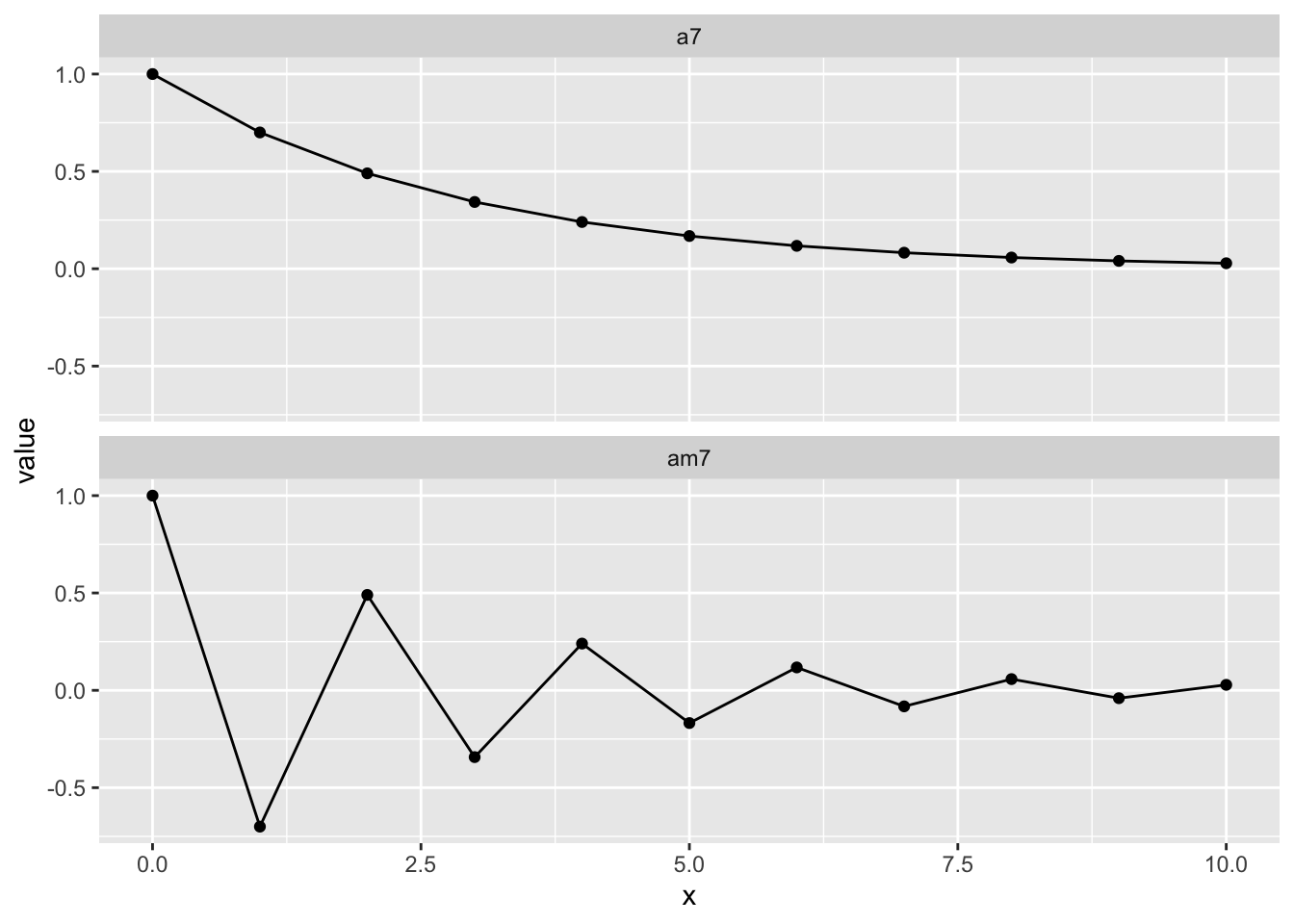
set.seed(1)
x <- w <- rnorm(100)
for (t in 2:100) x[t] <- 0.7 * x[t - 1] + w[t]
plot(x, type = "l")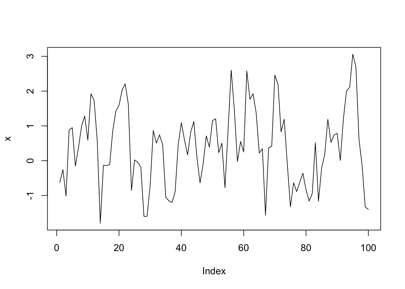
set.seed(1)
dat <- tibble(w = rnorm(100)) |>
    mutate(
        index = 1:n(),
         x = purrr::accumulate2(
            lag(w), w,
            \(acc, nxt, w) 0.7 * acc + w,
            .init = 0)[-1]) |>
    tsibble::as_tsibble(index = index)
autoplot(dat, .var = x)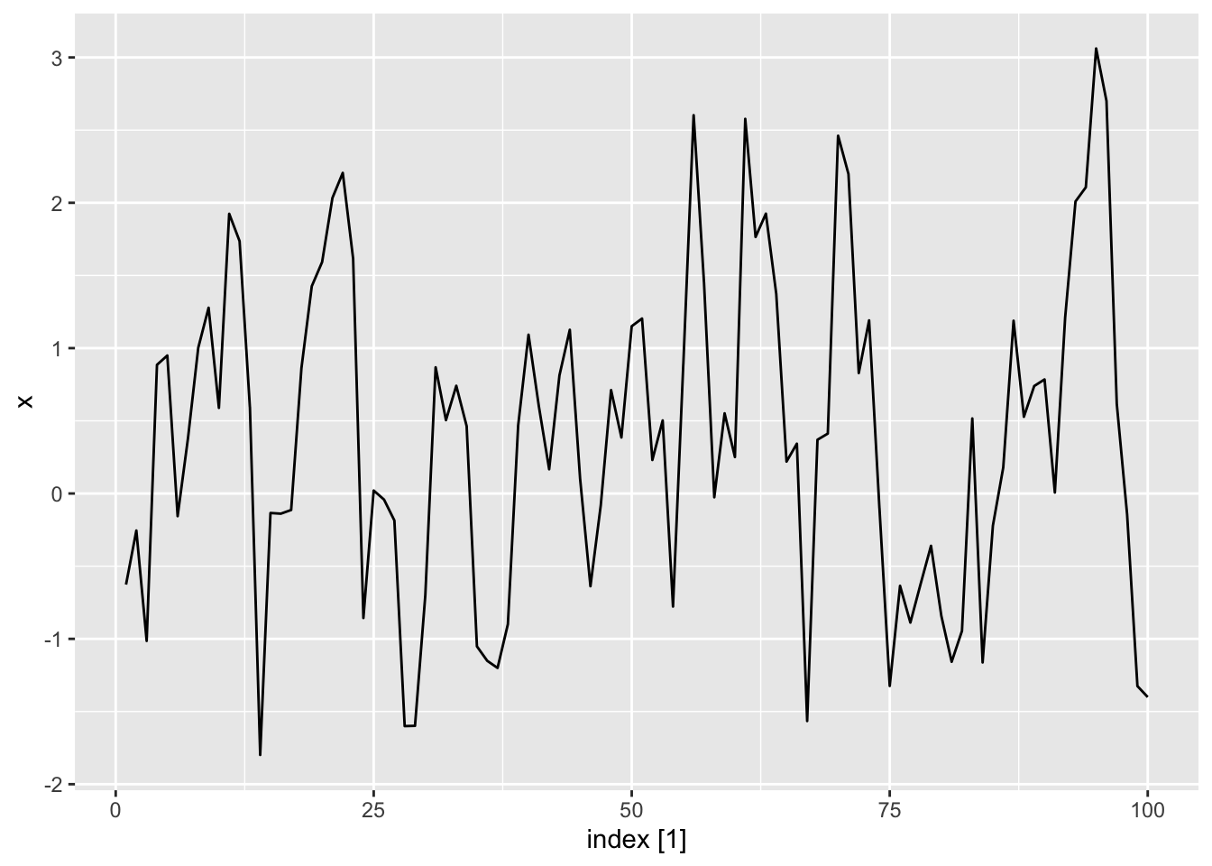
acf(x)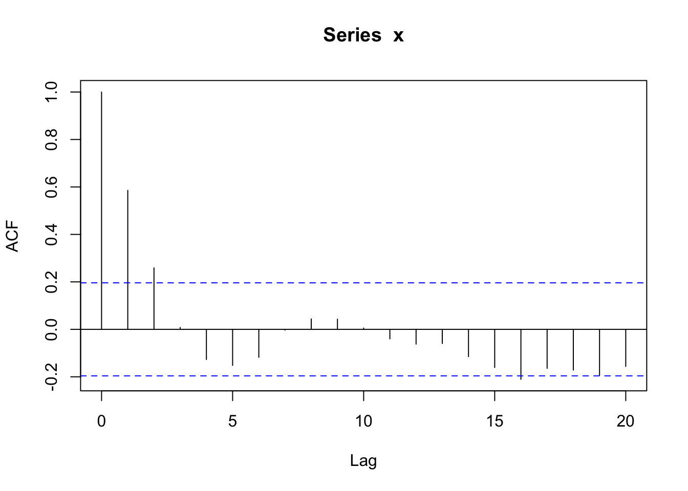
ACF(dat, x) |>
    autoplot()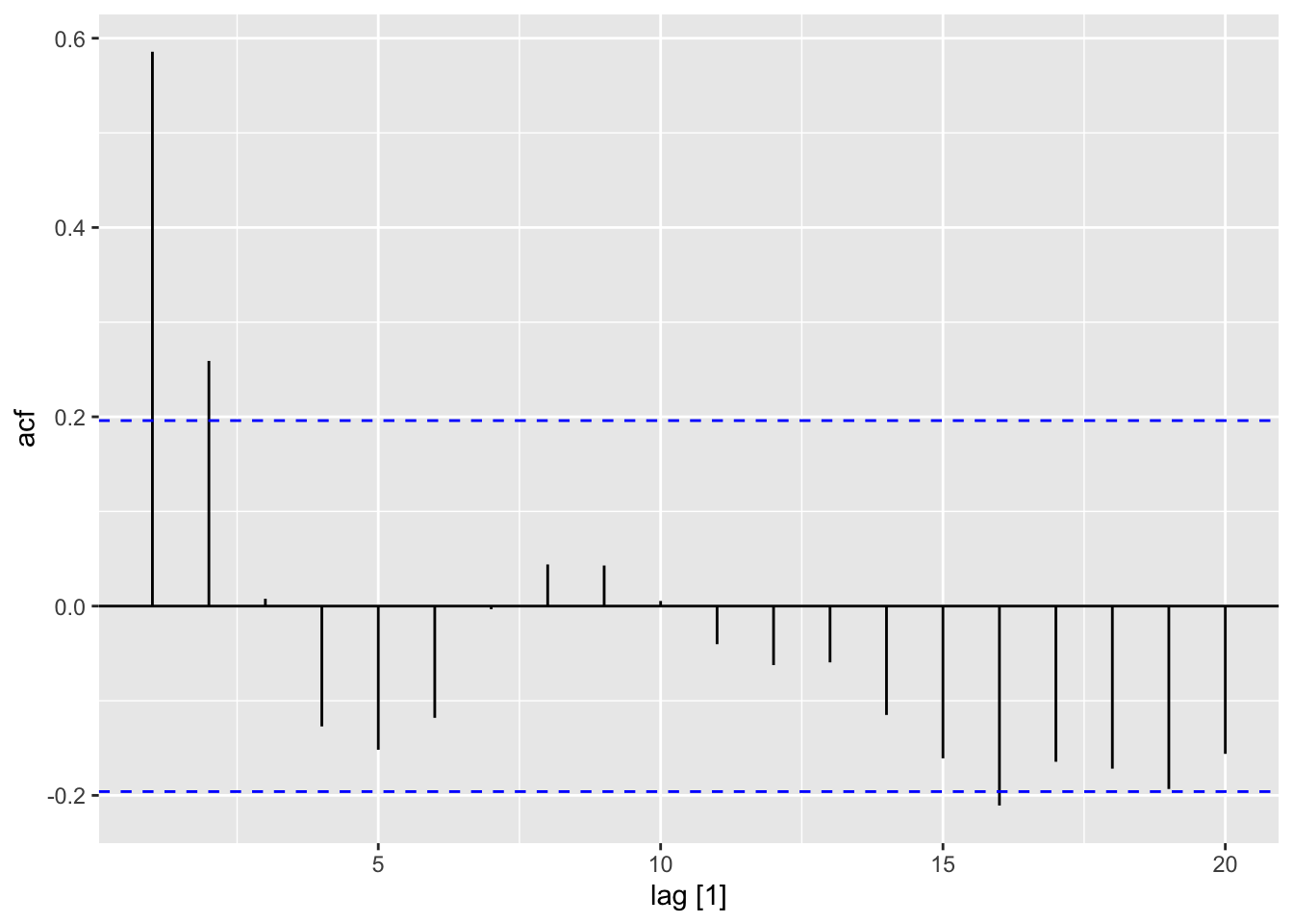
pacf(x)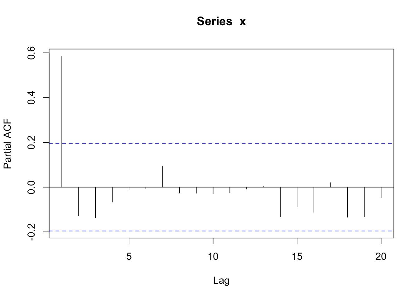
PACF(dat, x) |>
    autoplot()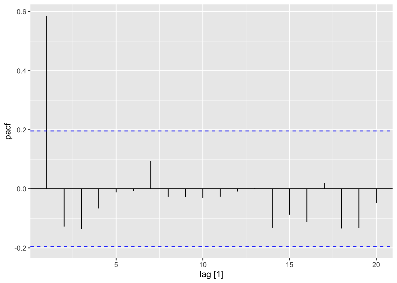
The stats::ar() and fable::AR() appear to have different optimization routines. For example, the fable::AR() model only allows optimization using Ordinary Least Squares (OLS), and stats::ar() provides multiple options. The textbook uses method = "mle" in these examples. Other differences are also apparent. As such, the results in the remaining sections do not match exactly.
Book code
set.seed(1)
x <- w <- rnorm(100)
for (t in 2:100) x[t] <- 0.7 * x[t - 1] + w[t]
x.ar <- ar(x, method = "mle")
x.ar$order
[1] 1Tidyverts code
set.seed(1)
dat <- tibble(w = rnorm(100)) |>
    mutate(
        index = 1:n(),
         x = purrr::accumulate2(
            lag(w), w,
            \(acc, nxt, w) 0.7 * acc + w,
            .init = 0)[-1]) |>
    tsibble::as_tsibble(index = index)
# Note that mle is not available using ols in ARMA
# answers slightly different
fit_ar <- dat |>
    model(AR(x ~ order(1)))
print("Order defined as 1 using order")
[1] "Order defined as 1 using order"x.ar$ar[1] 0.6009459tidy(fit_ar) |>
filter(str_detect(term, "ar")) |>
pull("estimate")[1] 0.6015796x.ar$ar + c(-2, 2) * sqrt(x.ar$asy.var)[1] # slight change[1] 0.4404031 0.7614886tidy(fit_ar) |>
mutate(
lb = estimate - 2 * std.error,
ub = estimate + 2 * std.error
)# A tibble: 2 × 8
.model term estimate std.error statistic p.value lb ub
<chr> <chr> <dbl> <dbl> <dbl> <dbl> <dbl> <dbl>
1 AR(x ~ order(1)) constant 0.157 0.0955 1.65 1.03e- 1 -0.0339 0.348
2 AR(x ~ order(1)) ar1 0.602 0.0814 7.39 5.03e-11 0.439 0.764set.seed(1)
dat <- tibble(w = rnorm(100)) |>
mutate(
index = 1:n(),
x = purrr::accumulate2(
lag(w), w,
\(acc, nxt, w) 0.7 * acc + w,
.init = 0)[-1]) |>
tsibble::as_tsibble(index = index)
# Note that mle is not available using ols in ARMA
# answers slightly different
fit_ar <- dat |>
model(AR(x ~ order(1)))
tidy(fit_ar) |>
    filter(str_detect(term, "ar")) |>
    pull("estimate")
tidy(fit_ar) |>
    mutate(
        lb = estimate - 2 * std.error,
        ub = estimate + 2 * std.error
)See note about stats::ar() and fable::AR() in previous section.
Book code
Z <- read.table("data/pounds_nz.dat", header = T)
Z.ts <- ts(Z, st = 1991, fr = 4)
Z.ar <- ar(Z.ts)
mean(Z.ts)
[1] 2.823251Tidyverts code
z <- read_table("data/pounds_nz.dat")
date_seq <- seq(
    lubridate::ymd("1991-01-01"),
    by = "3 months",
    length.out = nrow(z))
 z_ts <- z |>
    mutate(
        date = date_seq,
        quarter = tsibble::yearquarter(date)) |>
    as_tsibble(index = quarter)
z_ar <- z_ts |>
    model(AR(xrate ~ order(1)))
mean(z_ts$xrate)
[1] 2.823251c(Z.ar$order, Z.ar$ar)[1] 1.000000 0.890261tidy(z_ar) |>
filter(str_detect(term, "ar")) |>
pull("estimate")[1] 1.005271Z.ar$ar + c(-2, 2) * sqrt(Z.ar$asy.var)[1][1] 0.7405097 1.0400123tidy(z_ar) |>
mutate(
lb = estimate - 2 * std.error,
ub = estimate + 2 * std.error
)# A tibble: 1 × 8
.model term estimate std.error statistic p.value lb ub
<chr> <chr> <dbl> <dbl> <dbl> <dbl> <dbl> <dbl>
1 AR(xrate ~ order(1)) ar1 1.01 0.00781 129. 8.55e-52 0.990 1.02acf(Z.ar$res[-1])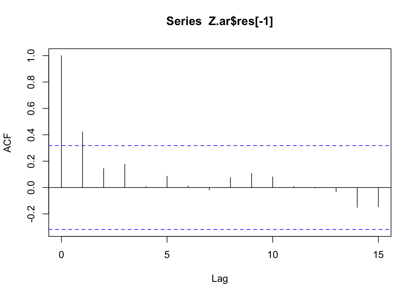
residuals(z_ar) |> ACF(y = .resid) |> autoplot()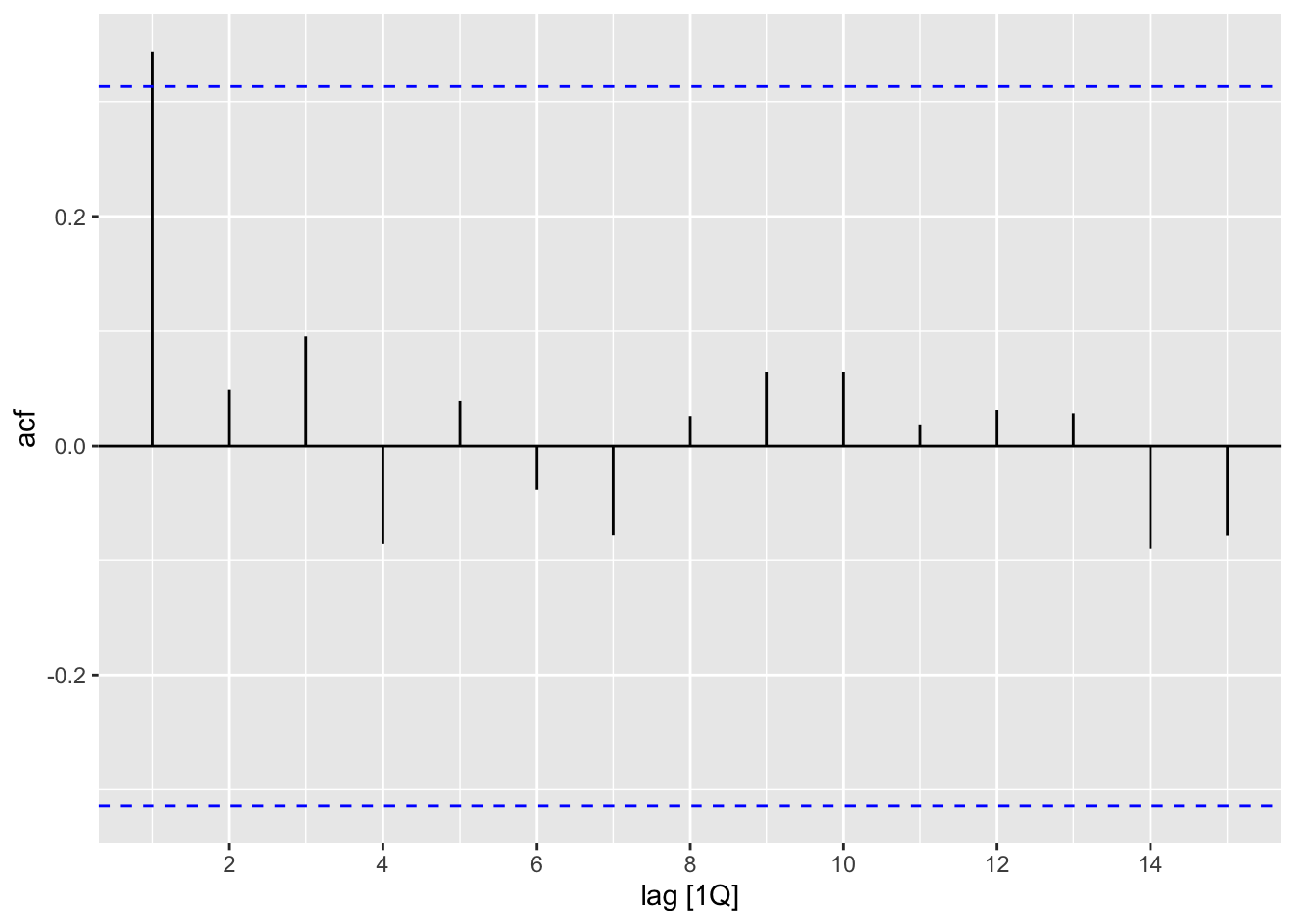
z <- read_table("data/pounds_nz.dat")
date_seq <- seq(
lubridate::ymd("1991-01-01"),
by = "3 months",
length.out = nrow(z))
z_ts <- z |>
mutate(
date = date_seq,
quarter = tsibble::yearquarter(date)) |>
as_tsibble(index = quarter)
z_ar <- z_ts |>
model(AR(xrate ~ order(1)))
mean(z_ts$xrate)
tidy(z_ar) |>
    filter(str_detect(term, "ar")) |>
    pull("estimate")
tidy(z_ar) |>
    mutate(
        lb = estimate - 2 * std.error,
        ub = estimate + 2 * std.error
    )
residuals(z_ar) |> ACF(y = .resid) |> autoplot()See note about stats::ar() and fable::AR() in previous section.
Book code
Global = scan("data/global.dat")
Global.ts = ts(Global, st = c(1856, 1), end = c(2005, 12),fr = 12)
Global.ar <- ar(aggregate(Global.ts, FUN = mean), method = "mle")
mean(aggregate(Global.ts, FUN = mean))
[1] -0.1382628Tidyverts code
global <- tibble(x = scan("data/global.dat")) |>
    mutate(
        date = seq(
            ymd("1856-01-01"),
            by = "1 months",
            length.out = n()),
        year = year(date),
        year_month = tsibble::yearmonth(date))

global_ts <- global |>
    as_tsibble(index = year_month)

global_ts_year <- global |>
    summarise(x = mean(x), .by = year) |>
    as_tsibble(index = year)

global_ar <- global_ts_year |>
    model(AR(x ~ order(1:9)))

mean(global_ts$x)
[1] -0.1382628Global.ar$order[1] 4tidy(global_ar) |> filter(str_detect(term, "ar")) |> nrow()[1] 4Global.ar$ar[1] 0.58762026 0.01260252 0.11116731 0.26763656tidy(global_ar) |> filter(str_detect(term, "ar")) |> pull(estimate)[1] 0.58176066 0.02164876 0.10747306 0.26707158acf(Global.ar$res[-(1:Global.ar$order)], lag = 50)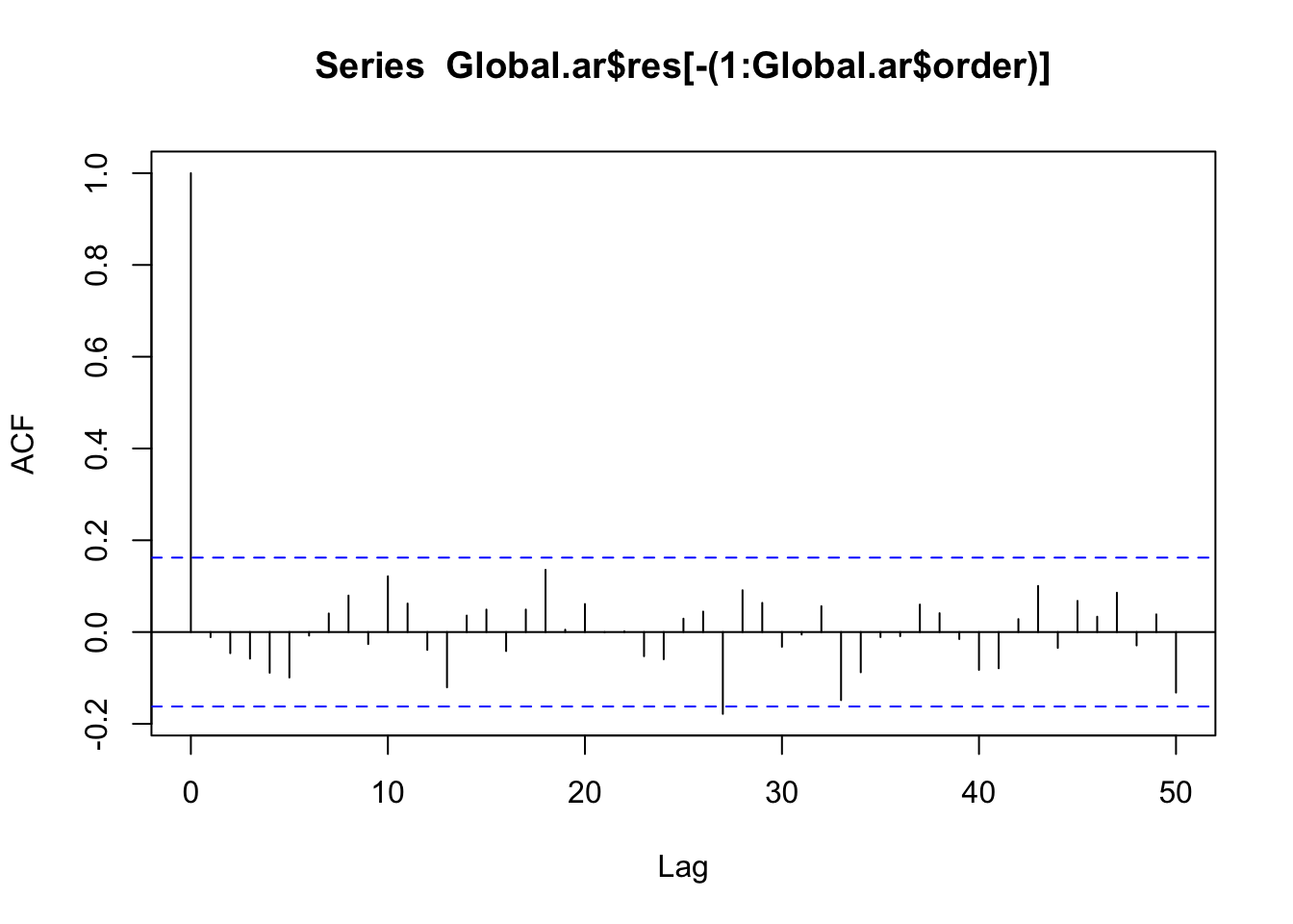
residuals(global_ar) |> ACF(lag_max = 50) |> autoplot()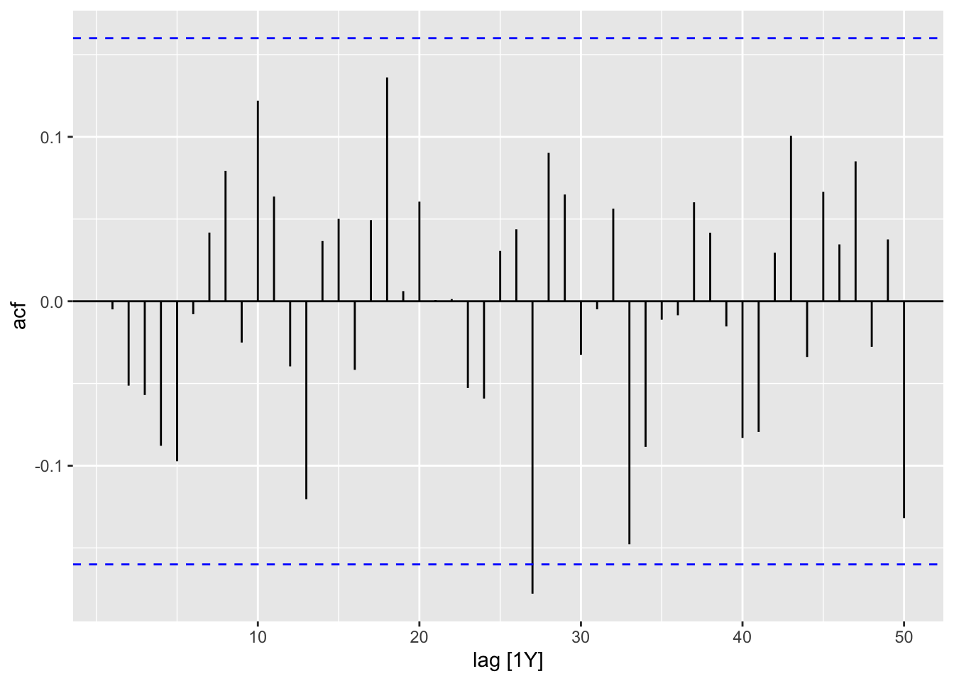
global <- tibble(x = scan("data/global.dat")) |>
    mutate(
        date = seq(
            ymd("1856-01-01"),
            by = "1 months",
            length.out = n()),
        year = year(date),
        year_month = tsibble::yearmonth(date))

global_ts <- global |>
    as_tsibble(index = year_month)

global_ts_year <- global |>
    summarise(x = mean(x), .by = year) |>
    as_tsibble(index = year)

global_ar <- global_ts_year |>
    model(AR(x ~ order(1:9)))

mean(global_ts$x)

tidy(global_ar) |> filter(str_detect(term, "ar")) |> nrow()

tidy(global_ar) |> filter(str_detect(term, "ar")) |> pull(estimate)

residuals(global_ar) |> ACF(lag_max = 50) |> autoplot()R commands used in examplesggplot2::geom_histogram(): Histograms and frequency polygonsggplot2::after_stat(): Control aesthetic evaluationdplyr::slice(): Subset rows using their positionsggplot2::facet_wrap(): Wrap a 1d ribbon of panels into 2dpurr::accumulate2(): Accumulate intermediate results of a vector reduction\():fable::AR(): Estimate a AR modelstats::residuals(): Extract Model Residuals