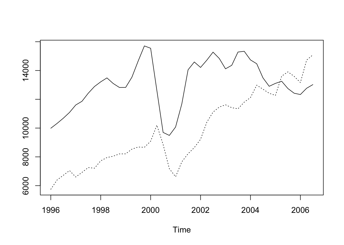
Businesses rely on forecasts of sales to plan production, justify marketing decisions, and guide research. A very efficient method of forecasting one variable is to find a related variable that leads it by one or more time intervals. The closer the relationship and the longer the lead time, the better this strategy becomes.
3.2.2 ‘Building Approvals’ Modern Look
Book code
<- read.table ("data/ApprovActiv.dat" , header= T)# attach(Build.dat) # bad practice <- ts (Build.dat$ Approvals, start = c (1996 ,1 ), freq= 4 )<- ts (Build.dat$ Activity, start = c (1996 ,1 ), freq= 4 )ts.plot (App.ts, Act.ts, lty = c (1 ,3 ))
Tidyverts code
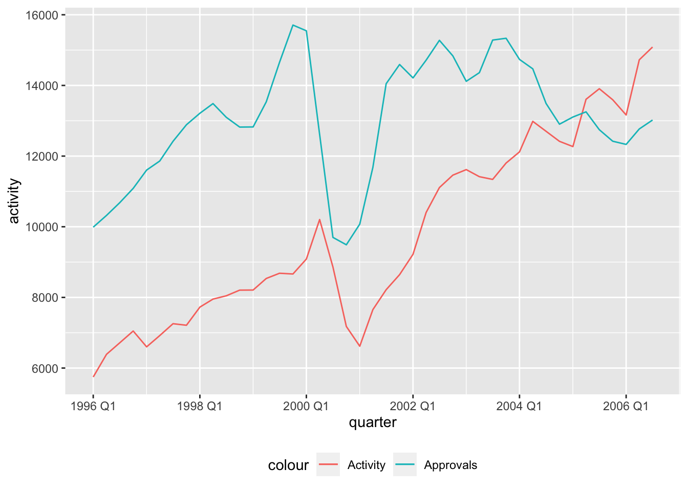
:: p_load ("tsibble" , "fable" , "feasts" ,"tsibbledata" , "fable.prophet" , "tidyverse" , "patchwork" )<- read_table ("data/ApprovActiv.dat" ) |> rename_all (str_to_lower) |> mutate (dates = seq (ymd ("1996-01-01" ), by = "3 months" , length.out = n ()),quarter = yearquarter (dates)) |> as_tsibble (index = quarter)ggplot (build_dat, aes (x = quarter)) + geom_line (aes (y = activity, color = "Activity" )) + geom_line (aes (y = approvals, color = "Approvals" )) + theme (legend.position = "bottom" )
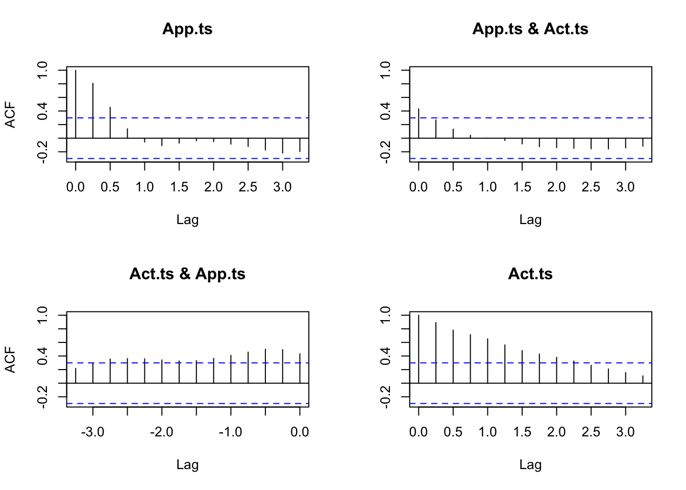
acf (ts.union (App.ts, Act.ts))
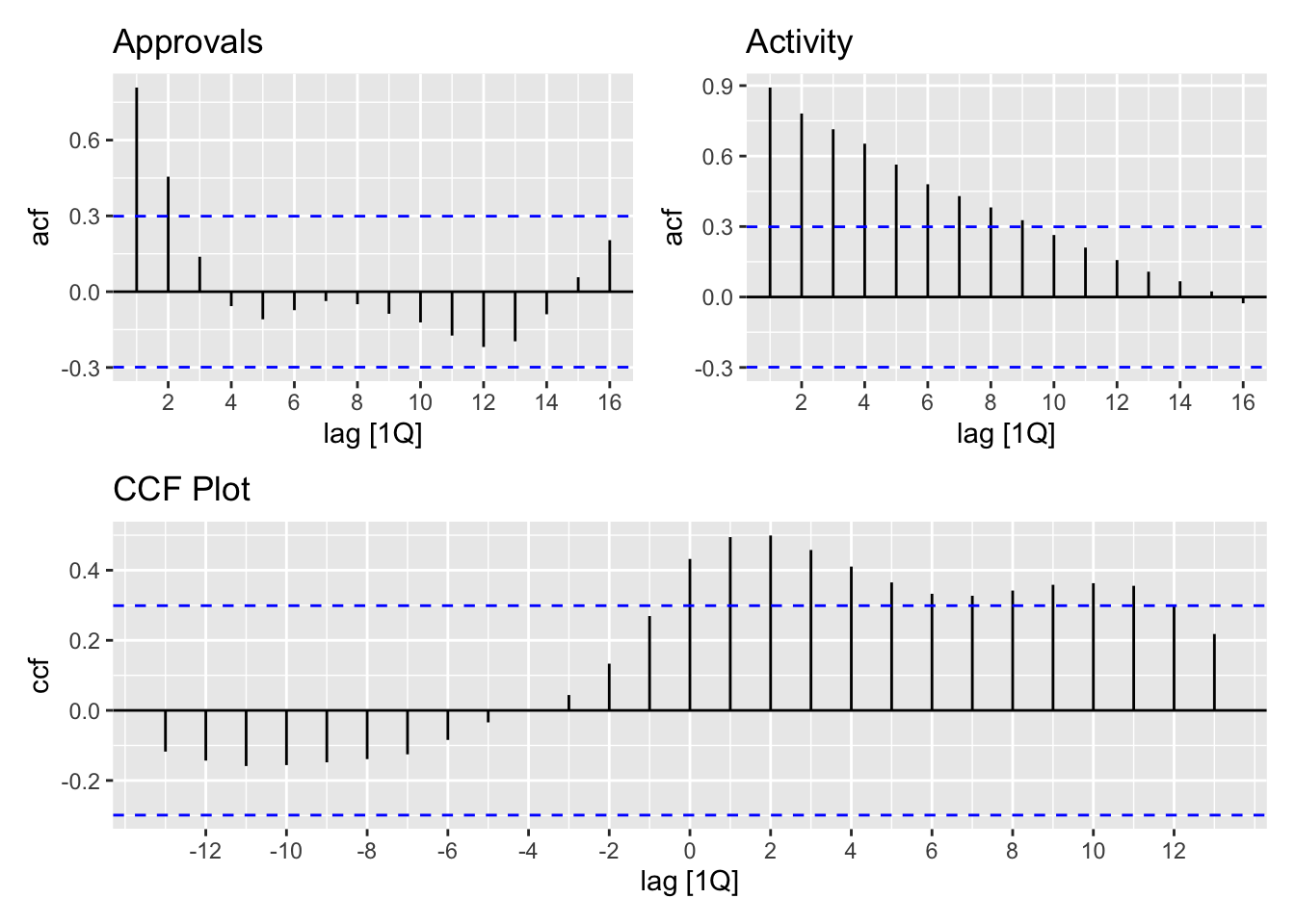
<- ACF (build_dat, y = approvals) |> autoplot () + labs (title = "Approvals" )<- ACF (build_dat, y = activity) |> autoplot () + labs (title = "Activity" )<- build_dat |> CCF (y = approvals, x = activity) |> autoplot () + labs (title = "CCF Plot" )+ acf_act) / joint_ccf_plot
print (acf (ts.union (App.ts, Act.ts), plot = FALSE ))
Autocorrelations of series 'ts.union(App.ts, Act.ts)', by lag

, , App.ts

 App.ts         Act.ts
  1.000 ( 0.00)  0.432 ( 0.00)
  0.808 ( 0.25)  0.494 (-0.25)
  0.455 ( 0.50)  0.499 (-0.50)
  0.138 ( 0.75)  0.458 (-0.75)
 -0.057 ( 1.00)  0.410 (-1.00)
 -0.109 ( 1.25)  0.365 (-1.25)
 -0.073 ( 1.50)  0.333 (-1.50)
 -0.037 ( 1.75)  0.327 (-1.75)
 -0.050 ( 2.00)  0.342 (-2.00)
 -0.087 ( 2.25)  0.358 (-2.25)
 -0.122 ( 2.50)  0.363 (-2.50)
 -0.174 ( 2.75)  0.356 (-2.75)
 -0.219 ( 3.00)  0.298 (-3.00)
 -0.196 ( 3.25)  0.218 (-3.25)

, , Act.ts

 App.ts         Act.ts
  0.432 ( 0.00)  1.000 ( 0.00)
  0.269 ( 0.25)  0.892 ( 0.25)
  0.133 ( 0.50)  0.781 ( 0.50)
  0.044 ( 0.75)  0.714 ( 0.75)
 -0.002 ( 1.00)  0.653 ( 1.00)
 -0.034 ( 1.25)  0.564 ( 1.25)
 -0.084 ( 1.50)  0.480 ( 1.50)
 -0.125 ( 1.75)  0.430 ( 1.75)
 -0.139 ( 2.00)  0.381 ( 2.00)
 -0.148 ( 2.25)  0.327 ( 2.25)
 -0.156 ( 2.50)  0.264 ( 2.50)
 -0.159 ( 2.75)  0.210 ( 2.75)
 -0.143 ( 3.00)  0.157 ( 3.00)
 -0.118 ( 3.25)  0.108 ( 3.25)
CCF (build_dat, approvals, activity)
# A tsibble: 27 x 2 [1Q]
        lag      ccf
   <cf_lag>    <dbl>
 1     -13Q -0.118
 2     -12Q -0.143
 3     -11Q -0.159
 4     -10Q -0.156
 5      -9Q -0.148
 6      -8Q -0.139
 7      -7Q -0.125
 8      -6Q -0.0843
 9      -5Q -0.0342
10      -4Q -0.00202
# ℹ 17 more rows
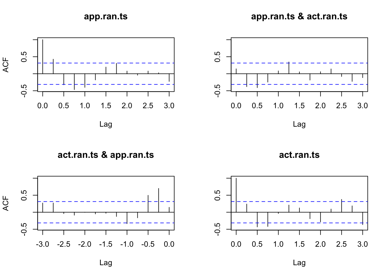
<- decompose (App.ts)$ random<- window (app.ran, start = c (1996 , 3 ), end = c (2006 ,1 )) # add end to fix <- decompose (Act.ts)$ random<- window (act.ran, start = c (1996 , 3 ), end = c (2006 ,1 )) # add end to fix acf (ts.union (app.ran.ts, act.ran.ts))
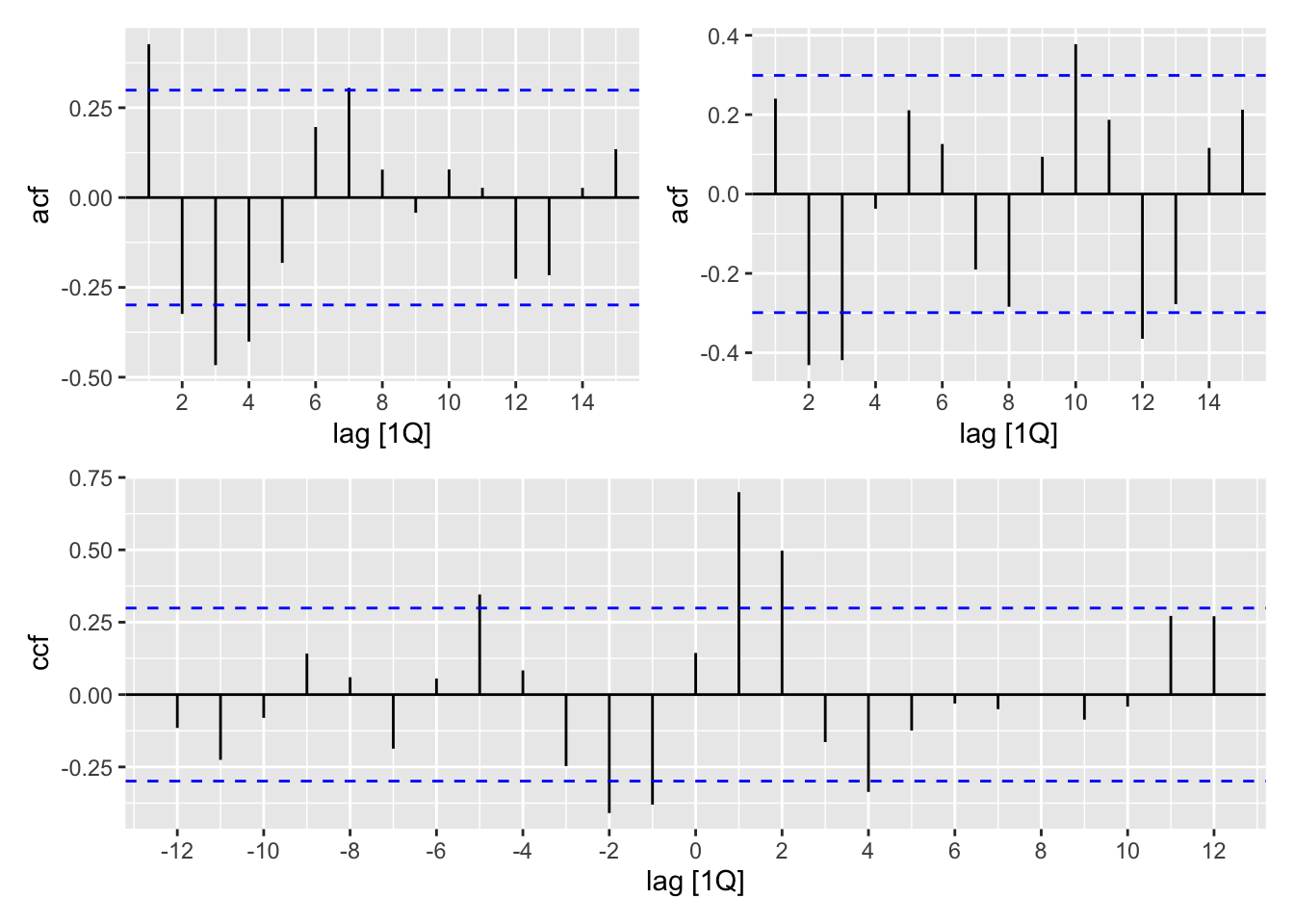
<- model (build_dat, feasts:: classical_decomposition (approvals)) |> components ()<- model (build_dat, feasts:: classical_decomposition (activity)) |> components ()<- ACF (app_decompose, random) |> autoplot ()<- ACF (act_decompose, random) |> autoplot ()<- select (app_decompose, quarter, random_app = random) |> left_join (select (act_decompose, quarter, random_act = random))<- random_decompose |> CCF (y = random_app, x = random_act) |> autoplot () + act_random) / joint_ccf_random
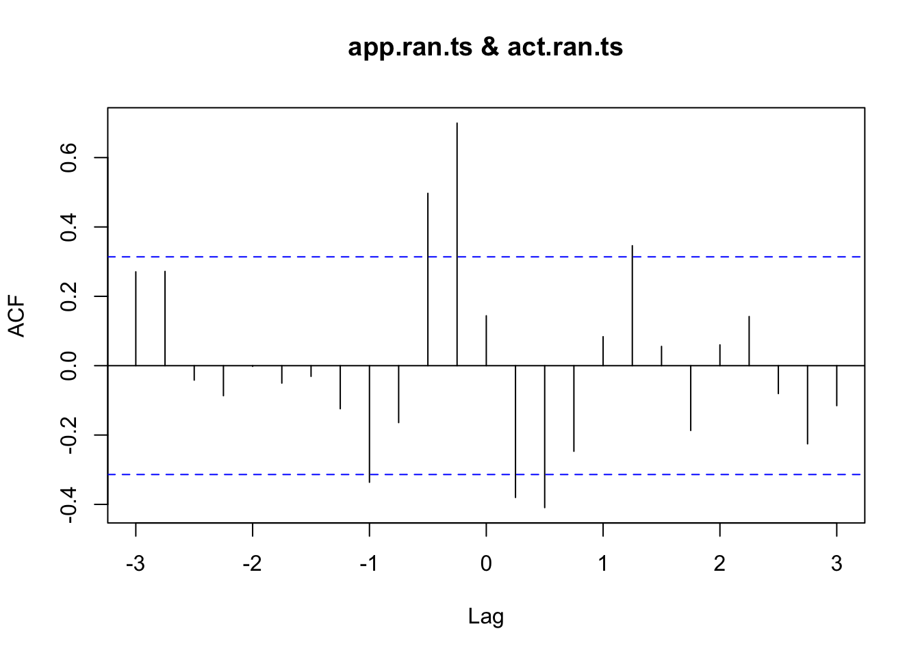
ccf (app.ran.ts, act.ran.ts)
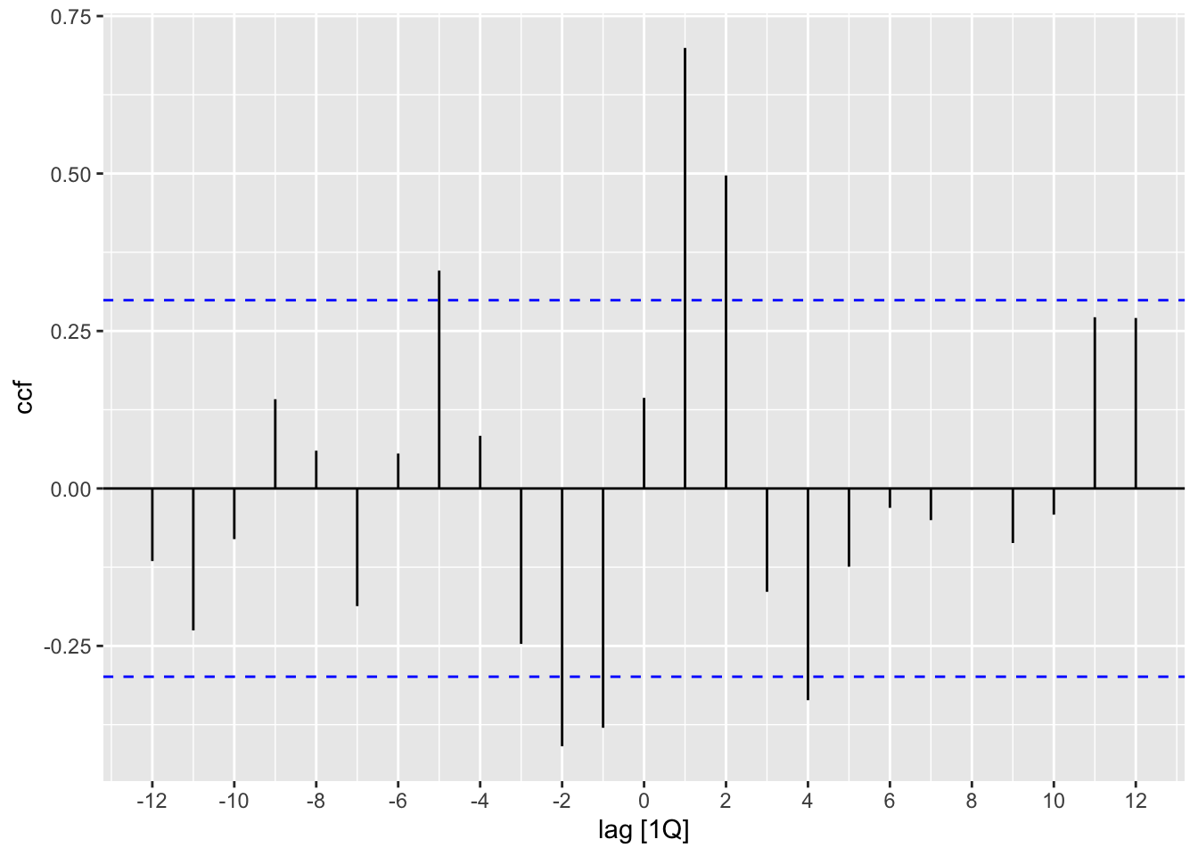
<- random_decompose |> CCF (y = random_app, x = random_act) |> autoplot ()
print (acf (ts.union (app.ran.ts, act.ran.ts), plot = FALSE ))
Autocorrelations of series 'ts.union(app.ran.ts, act.ran.ts)', by lag

, , app.ran.ts

 app.ran.ts     act.ran.ts
  1.000 ( 0.00)  0.144 ( 0.00)
  0.427 ( 0.25)  0.699 (-0.25)
 -0.324 ( 0.50)  0.497 (-0.50)
 -0.466 ( 0.75) -0.164 (-0.75)
 -0.401 ( 1.00) -0.336 (-1.00)
 -0.182 ( 1.25) -0.124 (-1.25)
  0.196 ( 1.50) -0.031 (-1.50)
  0.306 ( 1.75) -0.050 (-1.75)
  0.078 ( 2.00) -0.002 (-2.00)
 -0.042 ( 2.25) -0.087 (-2.25)
  0.078 ( 2.50) -0.042 (-2.50)
  0.027 ( 2.75)  0.272 (-2.75)
 -0.226 ( 3.00)  0.271 (-3.00)

, , act.ran.ts

 app.ran.ts     act.ran.ts
  0.144 ( 0.00)  1.000 ( 0.00)
 -0.380 ( 0.25)  0.240 ( 0.25)
 -0.409 ( 0.50) -0.431 ( 0.50)
 -0.247 ( 0.75) -0.419 ( 0.75)
  0.084 ( 1.00) -0.037 ( 1.00)
  0.346 ( 1.25)  0.211 ( 1.25)
  0.056 ( 1.50)  0.126 ( 1.50)
 -0.187 ( 1.75) -0.190 ( 1.75)
  0.060 ( 2.00) -0.284 ( 2.00)
  0.142 ( 2.25)  0.094 ( 2.25)
 -0.080 ( 2.50)  0.378 ( 2.50)
 -0.225 ( 2.75)  0.187 ( 2.75)
 -0.115 ( 3.00) -0.365 ( 3.00)
|> CCF (y = random_app, x = random_act)
# A tsibble: 25 x 2 [1Q]
        lag     ccf
   <cf_lag>   <dbl>
 1     -12Q -0.115
 2     -11Q -0.225
 3     -10Q -0.0804
 4      -9Q  0.142
 5      -8Q  0.0600
 6      -7Q -0.187
 7      -6Q  0.0556
 8      -5Q  0.346
 9      -4Q  0.0836
10      -3Q -0.247
# ℹ 15 more rows
Show the Book code in full
<- read.table ("data/ApprovActiv.dat" , header= T)# attach(Build.dat) # bad practice <- ts (Build.dat$ Approvals, start = c (1996 ,1 ), freq= 4 )<- ts (Build.dat$ Activity, start = c (1996 ,1 ), freq= 4 )ts.plot (App.ts, Act.ts, lty = c (1 ,3 ))acf (ts.union (App.ts, Act.ts))print (acf (ts.union (App.ts, Act.ts)))<- decompose (App.ts)$ random<- window (app.ran, start = c (1996 , 3 ), end = c (2006 ,1 )) # add end to fix <- decompose (Act.ts)$ random<- window (act.ran, start = c (1996 , 3 ), end = c (2006 ,1 )) # add end to fix acf (ts.union (app.ran.ts, act.ran.ts))ccf (app.ran.ts, act.ran.ts)print (acf (ts.union (app.ran.ts, act.ran.ts)))
Show the Tidyverts code in full
:: p_load ("tsibble" , "fable" , "feasts" ,"tsibbledata" , "fable.prophet" , "tidyverse" , "patchwork" )<- read_table ("data/ApprovActiv.dat" ) |> rename_all (str_to_lower) |> mutate (dates = seq (ymd ("1996-01-01" ), by = "3 months" , length.out = n ()),quarter = yearquarter (dates)) |> as_tsibble (index = quarter)ggplot (build_dat, aes (x = quarter)) + geom_line (aes (y = activity, color = "Activity" )) + geom_line (aes (y = approvals, color = "Approvals" )) + theme (legend.position = "bottom" )<- ACF (build_dat, y = approvals) |> autoplot () + labs (title = "Approvals" )<- ACF (build_dat, y = activity) |> autoplot () + labs (title = "Activity" )<- build_dat |> CCF (y = approvals, x = activity) |> autoplot () + labs (title = "CCF Plot" )+ acf_act) / joint_ccf_plotCCF (build_dat, approvals, activity)<- model (build_dat, feasts:: classical_decomposition (approvals)) |> components ()<- model (build_dat, feasts:: classical_decomposition (activity)) |> components ()<- ACF (app_decompose, random) |> autoplot ()<- ACF (act_decompose, random) |> autoplot ()<- select (app_decompose, quarter, random_app = random) |> left_join (select (act_decompose, quarter, random_act = random))<- random_decompose |> CCF (y = random_app, x = random_act) |> autoplot () + act_random) / joint_ccf_random<- random_decompose |> CCF (y = random_app, x = random_act) |> autoplot ()|> CCF (y = random_app, x = random_act)
The output from feasts::ACF() has a starkly different structure than the output of acf(). The following code snippet does additional wrangling to get the output in a more comparable format as shown below.
Explore Tidyverts code to match base R acf() output
<- read_table ("data/ApprovActiv.dat" ) |> rename_all (str_to_lower) |> mutate (dates = seq (ymd ("1996-01-01" ), by = "3 months" , length.out = n ()),quarter = yearquarter (dates)) |> pivot_longer (approvals: activity) |> as_tsibble (index = quarter, key = name)<- ACF (build_dat, y = value) |> pivot_wider (names_from = "name" ,values_from = "acf" ,names_prefix = "acf_" |> as_tibble () |> mutate (lag = as.character (lag)) |> bind_rows (tibble (lag = "0Q" , acf_activity = NA ,acf_approvals = NA <- build_dat |> pivot_wider (values_from = "value" , names_from = "name" ) |> CCF (y = approvals, x = activity) |> as_tibble () |> mutate (relation = ifelse (str_detect (lag, "-" ),"appTOact" , "actTOapp" ),lag = str_remove (lag, "-" )) |> pivot_wider (names_from = "relation" ,values_from = "ccf" ,names_prefix = "ccf_" ) |> mutate (ccf_appTOact = ifelse (is.na (ccf_appTOact), ccf_actTOapp, ccf_appTOact)left_join (ccf_dat, acf_dat) |> arrange (- row_number ()) |> select (acf_approvals, ccf_actTOapp, ccf_appTOact, acf_activity)
# A tibble: 14 × 4
   acf_approvals ccf_actTOapp ccf_appTOact acf_activity
           <dbl>        <dbl>        <dbl>        <dbl>
 1       NA             0.432      0.432         NA
 2        0.808         0.494      0.269          0.892
 3        0.455         0.499      0.133          0.781
 4        0.138         0.458      0.0439         0.714
 5       -0.0572        0.410     -0.00202        0.653
 6       -0.109         0.365     -0.0342         0.564
 7       -0.0731        0.333     -0.0843         0.480
 8       -0.0371        0.327     -0.125          0.430
 9       -0.0496        0.342     -0.139          0.381
10       -0.0874        0.358     -0.148          0.327
11       -0.122         0.363     -0.156          0.264
12       -0.174         0.356     -0.159          0.210
13       -0.219         0.298     -0.143          0.157
14       -0.196         0.218     -0.118          0.108
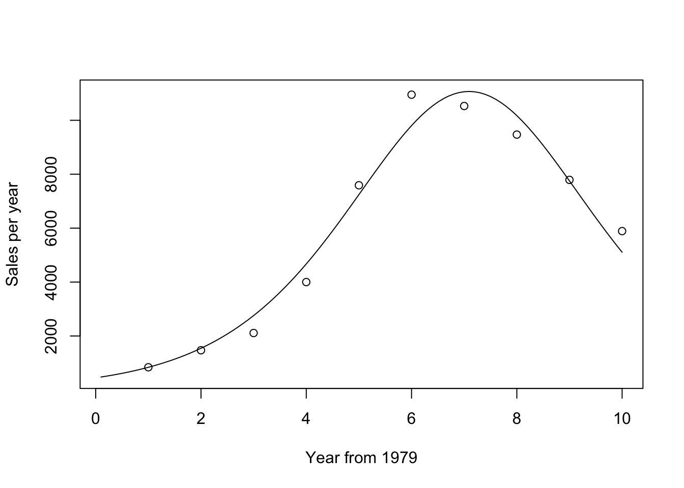
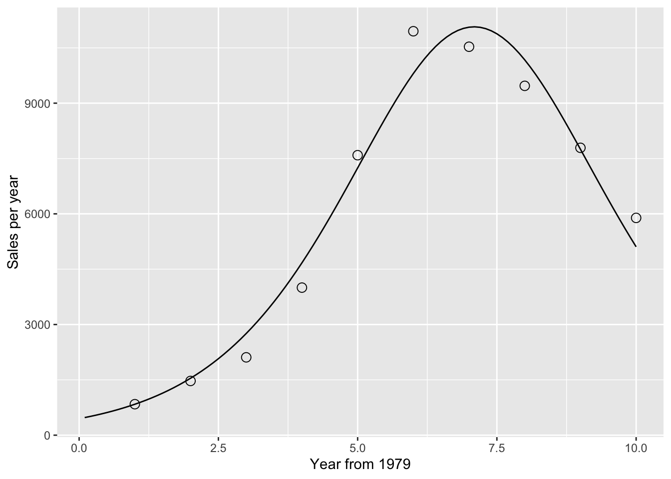
3.3.4 Bass Model Example Modern Look
Book code
<- 1 : 10 <- (1 : 100 ) / 10 <- c (840 ,1470 ,2110 ,4000 , 7590 , 10950 , 10530 , 9470 , 7790 , 5890 )<- cumsum (Sales)<- nls (Sales ~ M * ( ((P+ Q)^ 2 / P) * exp (- (P+ Q) * T79) ) / 1 + (Q/ P)* exp (- (P+ Q)* T79))^ 2 , start = list (M= 60630 , P= 0.03 , Q= 0.38 ))summary (Bass.nls)
Formula: Sales ~ M * (((P + Q)^2/P) * exp(-(P + Q) * T79))/(1 + (Q/P) *
    exp(-(P + Q) * T79))^2

Parameters:
   Estimate Std. Error t value Pr(>|t|)
M 6.798e+04  3.128e+03   21.74 1.10e-07 ***
P 6.594e-03  1.430e-03    4.61  0.00245 **
Q 6.381e-01  4.140e-02   15.41 1.17e-06 ***
---
Signif. codes:  0 '***' 0.001 '**' 0.01 '*' 0.05 '.' 0.1 ' ' 1

Residual standard error: 727.2 on 7 degrees of freedom

Number of iterations to convergence: 8
Achieved convergence tolerance: 7.395e-06
Tidyverts code
<- tibble (T79 = 1 : 10 ,Sales = c (840 ,1470 ,2110 ,4000 , 7590 , 10950 , 10530 , 9470 , 7790 , 5890 )) |> mutate (Cusales = cumsum (Sales))<- Sales ~ M * ( ((P+ Q)^ 2 / P) * exp (- (P+ Q) * T79) ) / (1 + (Q/ P)* exp (- (P+ Q)* T79))^ 2 <- nls (equation, data = dat, start = list (M= 60630 , P= 0.03 , Q= 0.38 ))summary (bass_nls)
Formula: Sales ~ M * (((P + Q)^2/P) * exp(-(P + Q) * T79))/(1 + (Q/P) *
    exp(-(P + Q) * T79))^2

Parameters:
   Estimate Std. Error t value Pr(>|t|)
M 6.798e+04  3.128e+03   21.74 1.10e-07 ***
P 6.594e-03  1.430e-03    4.61  0.00245 **
Q 6.381e-01  4.140e-02   15.41 1.17e-06 ***
---
Signif. codes:  0 '***' 0.001 '**' 0.01 '*' 0.05 '.' 0.1 ' ' 1

Residual standard error: 727.2 on 7 degrees of freedom

Number of iterations to convergence: 8
Achieved convergence tolerance: 7.395e-06
<- coef (Bass.nls)<- Bcoef[1 ]<- Bcoef[2 ]<- Bcoef[3 ]<- exp (- (p+ q) * Tdelt)<- m * ( (p+ q)^ 2 / p ) * ngete / (1 + (q/ p) * ngete)^ 2 plot (Tdelt, Bpdf,xlab = "Year from 1979" ,ylab = "Sales per year" , type= 'l' )points (T79, Sales)
<- tibble (tdelt = (1 : 100 ) / 10 ,m = coef (bass_nls)["M" ],p = coef (bass_nls)["P" ],q = coef (bass_nls)["Q" ]) |> mutate (ngete = exp (- (p+ q) * tdelt),bpdf = m * ( (p+ q)^ 2 / p ) * ngete / (1 + (q/ p) * ngete)^ 2 )ggplot (pdat, aes (x = tdelt, y = bpdf)) + geom_line () + geom_point (data = dat,aes (x = T79, y = Sales),size = 3 , shape = 1 ) + labs (x = "Year from 1979" , y = "Sales per year" )
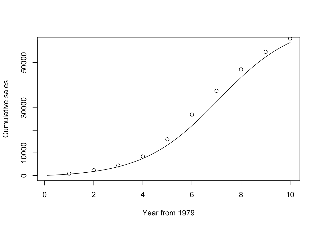
<- m * (1 - ngete)/ (1 + (q/ p)* ngete)plot (Tdelt, Bcdf,xlab = "Year from 1979" ,ylab = "Cumulative sales" , type= 'l' )points (T79, Cusales)
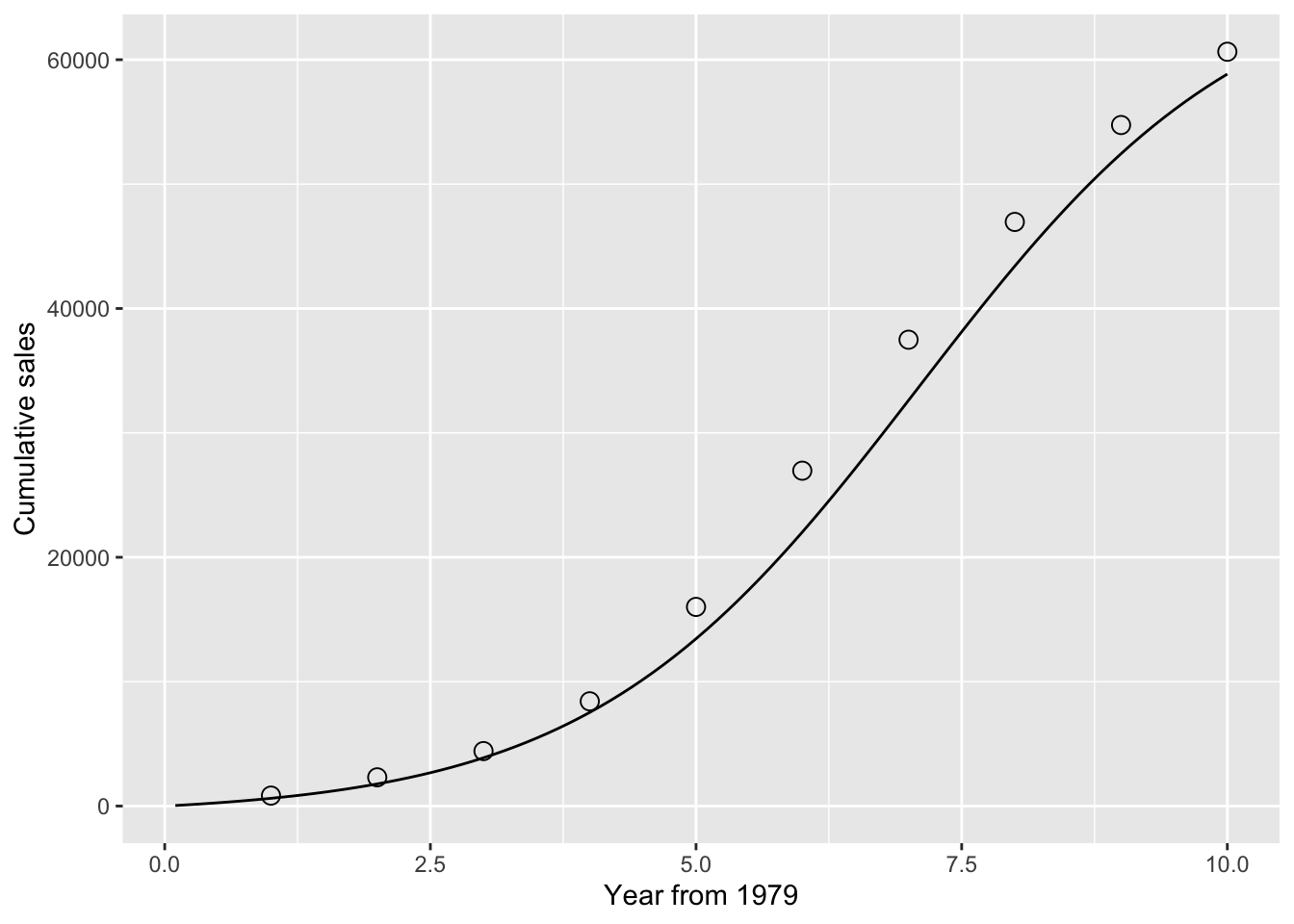
<- mutate (pdat, bcdf = m * (1 - ngete)/ (1 + (q/ p) * ngete))ggplot (pdat, aes (x = tdelt, y = bcdf)) + geom_line () + geom_point (data = dat,aes (x = T79, y = Cusales),size = 3 , shape = 1 ) + labs (x = "Year from 1979" ,y = "Cumulative sales" )
Show the Book code in full
<- 1 : 10 <- (1 : 100 ) / 10 <- c (840 ,1470 ,2110 ,4000 , 7590 , 10950 , 10530 , 9470 , 7790 , 5890 )<- cumsum (Sales)<- nls (Sales ~ M * ( ((P+ Q)^ 2 / P) * exp (- (P+ Q) * T79) ) / 1 + (Q/ P)* exp (- (P+ Q)* T79))^ 2 , start = list (M= 60630 , P= 0.03 , Q= 0.38 ))summary (Bass.nls)<- coef (Bass.nls)<- Bcoef[1 ]<- Bcoef[2 ]<- Bcoef[3 ]<- exp (- (p+ q) * Tdelt)<- m * ( (p+ q)^ 2 / p ) * ngete / (1 + (q/ p) * ngete)^ 2 plot (Tdelt, Bpdf,xlab = "Year from 1979" ,ylab = "Sales per year" , type= 'l' )points (T79, Sales)<- m * (1 - ngete)/ (1 + (q/ p)* ngete)plot (Tdelt, Bcdf,xlab = "Year from 1979" ,ylab = "Cumulative sales" , type= 'l' )points (T79, Cusales)
Show the Tidyverts code in full
<- tibble (T79 = 1 : 10 ,Sales = c (840 ,1470 ,2110 ,4000 , 7590 , 10950 , 10530 , 9470 , 7790 , 5890 )) |> mutate (Cusales = cumsum (Sales))<- Sales ~ M * ( ((P+ Q)^ 2 / P) * exp (- (P+ Q) * T79) ) / (1 + (Q/ P)* exp (- (P+ Q)* T79))^ 2 <- nls (equation, data = dat, start = list (M= 60630 , P= 0.03 , Q= 0.38 ))summary (bass_nls)<- tibble (tdelt = (1 : 100 ) / 10 ,m = coef (bass_nls)["M" ],p = coef (bass_nls)["P" ],q = coef (bass_nls)["Q" ]) |> mutate (ngete = exp (- (p+ q) * tdelt),bpdf = m * ( (p+ q)^ 2 / p ) * ngete / (1 + (q/ p) * ngete)^ 2 )ggplot (pdat, aes (x = tdelt, y = bpdf)) + geom_line () + geom_point (data = dat,aes (x = T79, y = Sales),size = 3 , shape = 1 ) + labs (x = "Year from 1979" , y = "Sales per year" )<- mutate (pdat, bcdf = m * (1 - ngete)/ (1 + (q/ p) * ngete))ggplot (pdat, aes (x = tdelt, y = bcdf)) + geom_line () + geom_point (data = dat,aes (x = T79, y = Cusales),size = 3 , shape = 1 ) + labs (x = "Year from 1979" , y = "Cumulative sales" )
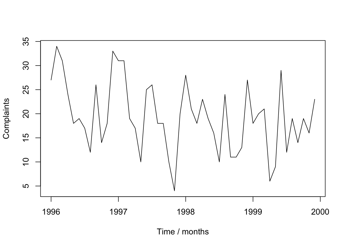
3.4.1 “Exponential smoothing” and “Complaints” Modern Look
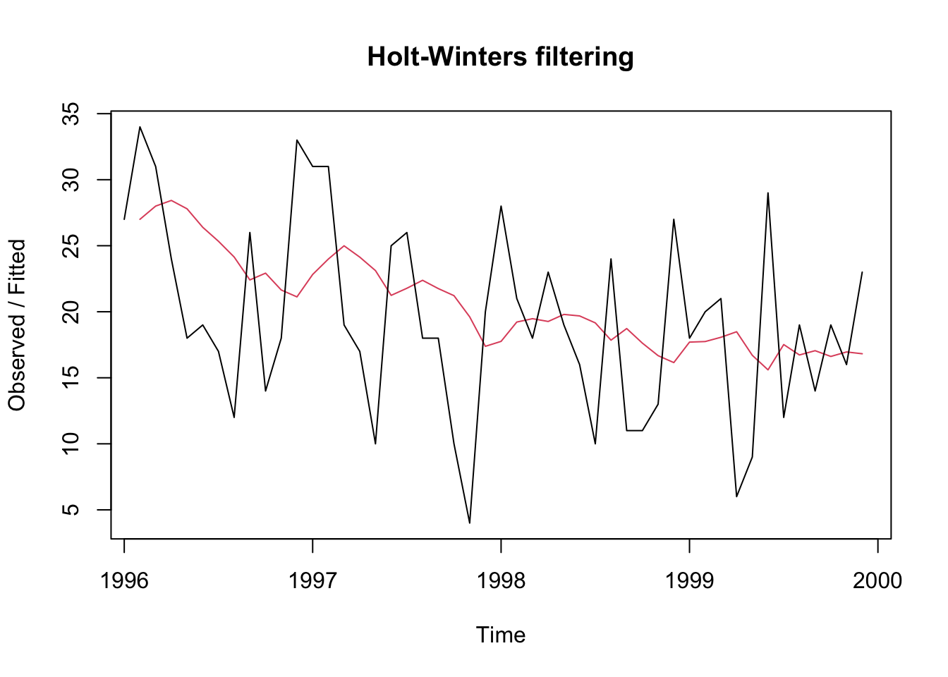
The HoltWinters methods do not return the same results between the HoltWinters() and the feasts::model(ETS()) methods. It appears that the estimation methods used within each package to implement the HoltWinters methods differ slightly.
Book code
<- read.table ("data/motororg.dat" , header = T)# attach(Motor.dat) # bad practice <- ts (Motor.dat$ complaints, start = c (1996 , 1 ), freq = 12 )plot (Comp.ts, xlab = "Time / months" , ylab = "Complaints" )
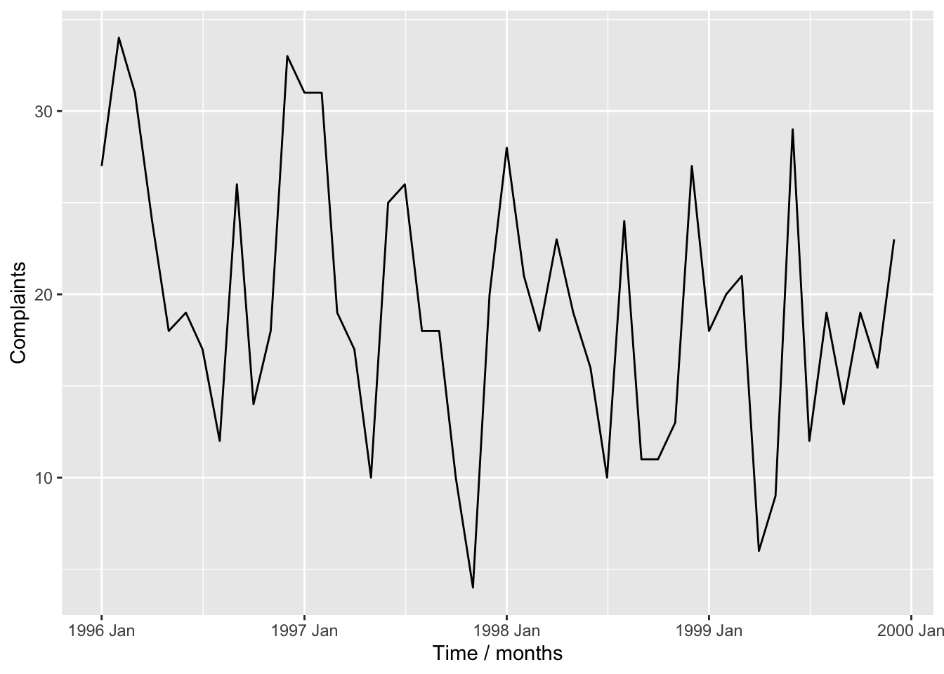
Tidyverts code
<- read_table ("data/motororg.dat" ) |> mutate (dates = seq (ymd ("1996-01-01" ), by = "1 months" ,length.out = n ()),months = yearmonth (dates)<- as_tsibble (motor_dat, index = months)autoplot (comp_ts) + labs (x = "Time / months" , y = "Complaints" )
<- HoltWinters (Comp.ts,beta = FALSE , gamma = FALSE )) # edits to book code
Holt-Winters exponential smoothing without trend and without seasonal component.

Call:
HoltWinters(x = Comp.ts, beta = FALSE, gamma = FALSE)

Smoothing parameters:
 alpha: 0.1429622
 beta : FALSE
 gamma: FALSE

Coefficients:
      [,1]
a 17.70343
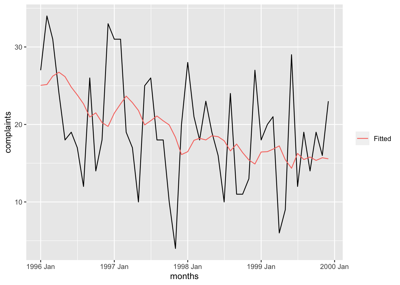
<- comp_ts |> model (Additive = ETS (complaints ~ trend ("A" , alpha = 0.1429622 , beta = 0 ) + error ("A" ) + season ("N" ),opt_crit = "amse" , nmse = 1 ))report (comp_hw1)
Series: complaints
Model: ETS(A,A,N)
  Smoothing parameters:
    alpha = 0.1429622
    beta  = 0

  Initial states:
     l[0]       b[0]
 25.22968 -0.1790294

  sigma^2:  54.8316

     AIC     AICc      BIC
379.8459 380.3914 385.4595
augment (comp_hw1) |> ggplot (aes (x = months, y = complaints)) + geom_line () + geom_line (aes (y = .fitted, color = "Fitted" )) + labs (color = "" )
sum (components (comp_hw1)$ remainder^ 2 , na.rm = T)
<- HoltWinters (Comp.ts, alpha = 0.2 ,beta = FALSE , gamma = FALSE ) # edits to book code $ SSE
<- comp_ts |> model (Additive = ETS (complaints ~ trend ("A" , alpha = 0.2 , beta = 0 ) + error ("A" ) + season ("N" ),opt_crit = "amse" , nmse = 1 ))sum (components (comp_hw2)$ remainder^ 2 , na.rm = T)
Show the Book code in full
#https://rpubs.com/pg2000in/TimeSeries5 <- read.table ("data/motororg.dat" , header = T)# attach(Motor.dat) # bad practice <- ts (Motor.dat$ complaints,start = c (1996 , 1 ),freq = 12 )plot (Comp.ts,xlab = "Time / months" ,ylab = "Complaints" )<- HoltWinters (Comp.ts,beta = FALSE , gamma = FALSE ) # edits to book code plot (Comp.hw1)$ SSE<- HoltWinters (Comp.ts, alpha = 0.2 ,beta = FALSE , gamma = FALSE ) # edits to book code $ SSE
Show the Tidyverts code in full
<- read_table ("data/motororg.dat" ) |> mutate (dates = seq (ymd ("1996-01-01" ), by = "1 months" ,length.out = n ()),months = yearmonth (dates)<- as_tsibble (motor_dat, index = months)autoplot (comp_ts) + labs (x = "Time / months" , y = "Complaints" )<- comp_ts |> model (Additive = ETS (complaints ~ trend ("A" , alpha = 0.1429622 , beta = 0 ) + error ("A" ) + season ("N" ),opt_crit = "amse" , nmse = 1 ))augment (comp_hw1) |> ggplot (aes (x = months, y = complaints)) + geom_line () + geom_line (aes (y = .fitted, color = "Fitted" )) + labs (color = "" )<- comp_ts |> model (Additive = ETS (complaints ~ trend ("A" , alpha = 0.2 , beta = 0 ) + error ("A" ) + season ("N" ),opt_crit = "amse" , nmse = 1 ))sum (components (comp_hw2)$ remainder^ 2 , na.rm = T)
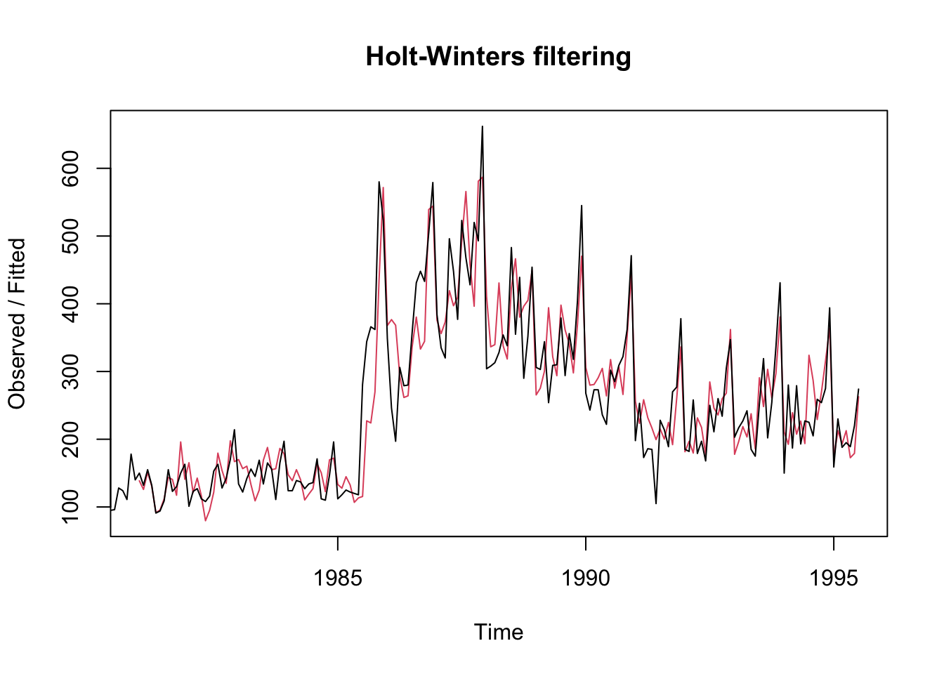
3.4.2 “Holt-Winters” and “Australian wine” Modern Look
Book code
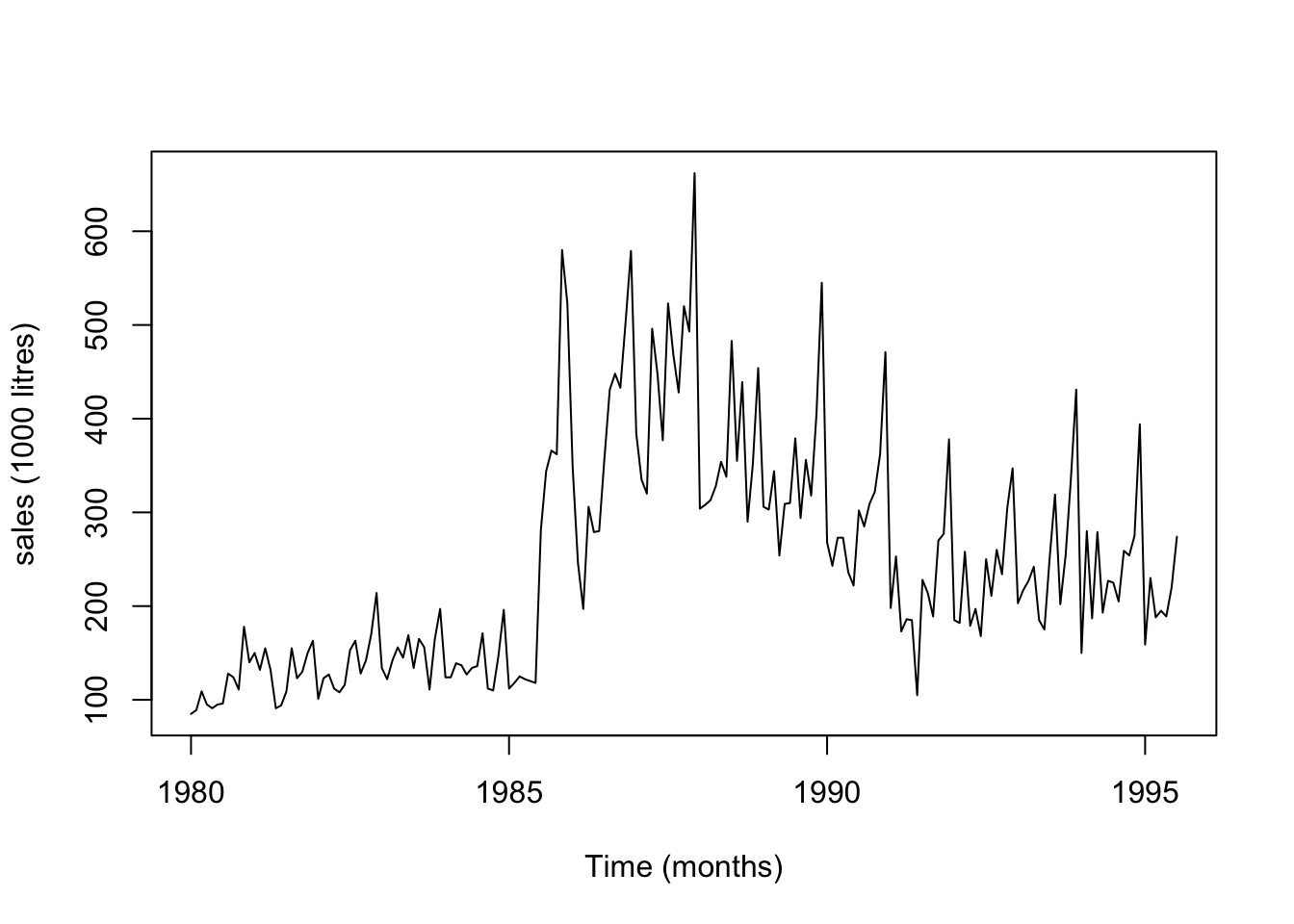
<- read.table ("data/wine.dat" , header = T)# attach (wine.dat) # bad practice <- ts (wine.dat$ sweetw, start = c (1980 ,1 ), freq = 12 )plot (sweetw.ts, xlab= "Time (months)" , ylab = "sales (1000 litres)" )
Tidyverts code
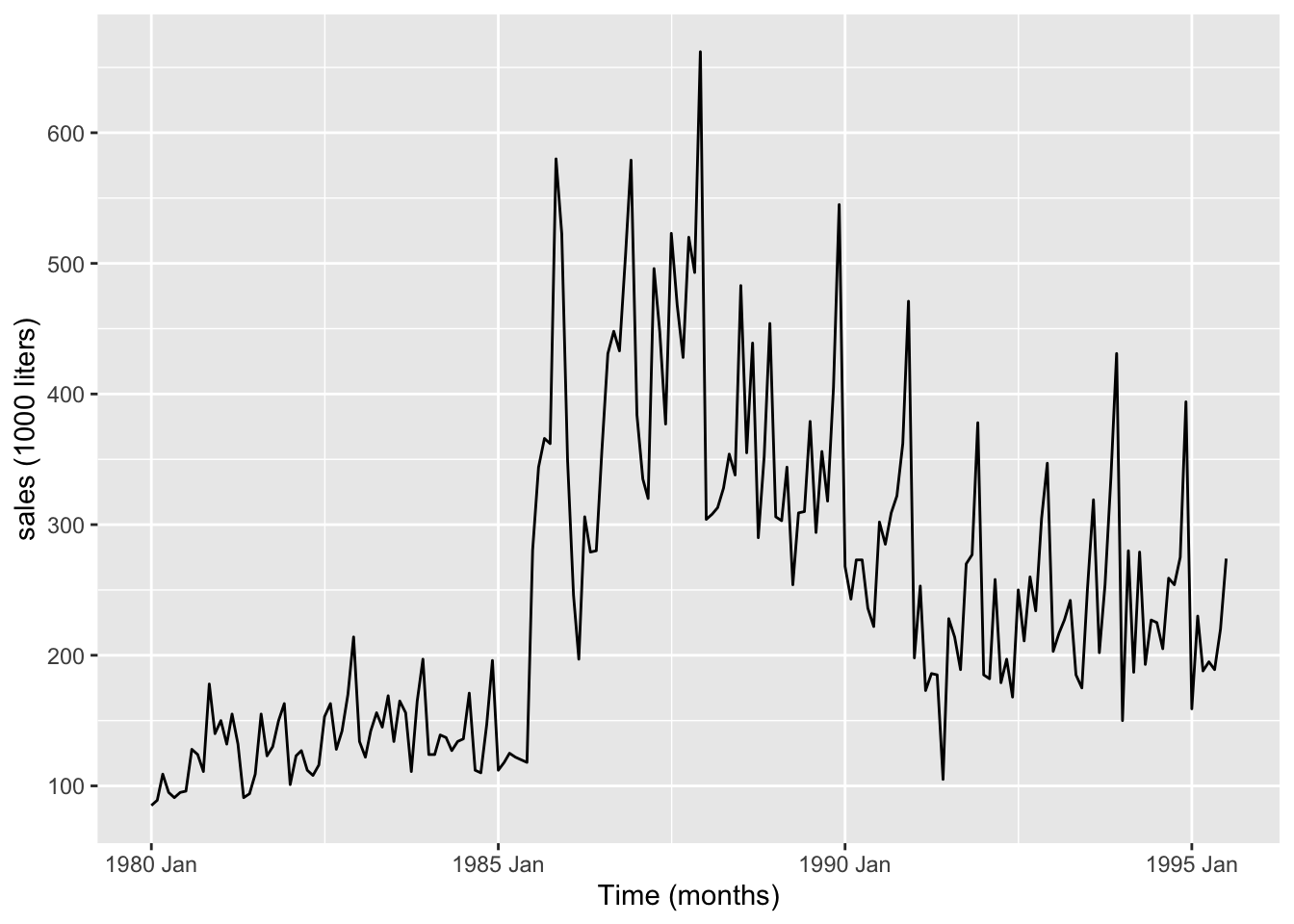
<- read_table ("data/wine.dat" ) |> mutate (dates = seq (ymd ("1980-01-01" ), by = "1 months" ,length.out = n ()),months = yearmonth (dates)<- as_tsibble (select (wine_dat, sweetw, months),index = months)autoplot (sweetw_ts) + labs (x = "Time (months)" ,y = "sales (1000 liters)" )
<- HoltWinters (sweetw.ts, seasonal = "multiplicative" ) #not quite the same as book
Holt-Winters exponential smoothing with trend and multiplicative seasonal component.

Call:
HoltWinters(x = sweetw.ts, seasonal = "multiplicative")

Smoothing parameters:
 alpha: 0.4086698
 beta : 0
 gamma: 0.4929402

Coefficients:
           [,1]
a   285.6890314
b     1.3509615
s1    0.9498541
s2    0.9767623
s3    1.0275900
s4    1.1991924
s5    1.5463100
s6    0.6730235
s7    0.8925981
s8    0.7557814
s9    0.8227500
s10   0.7241711
s11   0.7434861
s12   0.9472648
<- sweetw_ts |> model (Multiplicative = ETS (sweetw ~ trend ("M" ) + error ("A" ) + season ("M" ),opt_crit = "amse" , nmse = 1 ))report (sweetw_hw)
Series: sweetw
Model: ETS(A,M,M)
  Smoothing parameters:
    alpha = 0.4286965
    beta  = 0.0001905936
    gamma = 0.0001968977

  Initial states:
     l[0]      b[0]     s[0]    s[-1]     s[-2]   s[-3]    s[-4]    s[-5]
 112.0738 0.9962457 1.495189 1.246035 0.9870751 1.03928 1.008875 1.078576
     s[-6]     s[-7]     s[-8]     s[-9]    s[-10]    s[-11]
 0.8232773 0.8637861 0.9308562 0.8717047 0.8427252 0.8126209

  sigma^2:  2116.25

     AIC     AICc      BIC
2427.425 2431.046 2482.354
          a           b          s1          s2          s3          s4
285.6890314   1.3509615   0.9498541   0.9767623   1.0275900   1.1991924
         s5          s6          s7          s8          s9         s10
  1.5463100   0.6730235   0.8925981   0.7557814   0.8227500   0.7241711
        s11         s12
  0.7434861   0.9472648
# A tibble: 17 × 3
   .model         term     estimate
   <chr>          <chr>       <dbl>
 1 Multiplicative alpha    0.429
 2 Multiplicative beta     0.000191
 3 Multiplicative gamma    0.000197
 4 Multiplicative l[0]   112.
 5 Multiplicative b[0]     0.996
 6 Multiplicative s[0]     1.50
 7 Multiplicative s[-1]    1.25
 8 Multiplicative s[-2]    0.987
 9 Multiplicative s[-3]    1.04
10 Multiplicative s[-4]    1.01
11 Multiplicative s[-5]    1.08
12 Multiplicative s[-6]    0.823
13 Multiplicative s[-7]    0.864
14 Multiplicative s[-8]    0.931
15 Multiplicative s[-9]    0.872
16 Multiplicative s[-10]   0.843
17 Multiplicative s[-11]   0.813
sum (components (sweetw_hw)$ remainder^ 2 , na.rm = T)
sqrt (sweetw.hw$ SSE/ length (wine.dat$ sweetw)) # book has 50.04
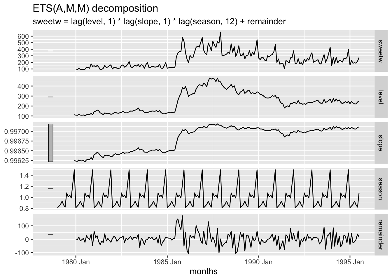
autoplot (components (sweetw_hw))
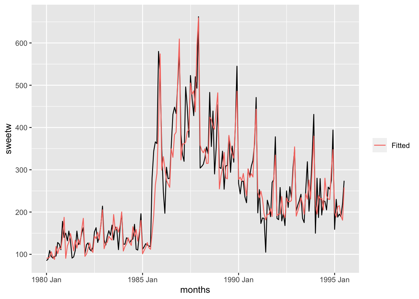
augment (sweetw_hw) |> ggplot (aes (x = months, y = sweetw)) + geom_line () + geom_line (aes (y = .fitted, color = "Fitted" )) + labs (color = "" )
Show the Book code in full
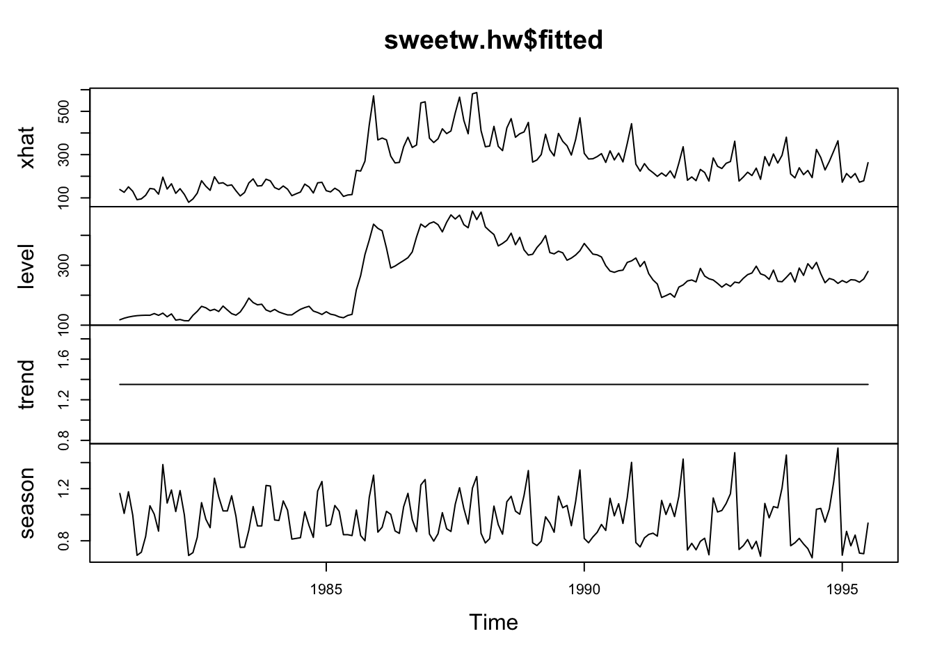
# https://otexts.com/fpp2/holt-winters.html <- read.table ("data/wine.dat" , header = T)# attach (wine.dat) # bad practice <- ts (wine.dat$ sweetw, start = c (1980 ,1 ), freq = 12 )plot (sweetw.ts, xlab= "Time (months)" , ylab = "sales (1000 litres)" )<- HoltWinters (sweetw.ts, seasonal = "multiplicative" ) #not quite the same as book $ coef$ SSEsqrt (sweetw.hw$ SSE/ length (wine.dat$ sweetw)) # book has 50.04 sd (wine.dat$ sweetw)plot (sweetw.hw$ fitted)plot (sweetw.hw)
Show the Tidyverts code in full
<- read_table ("data/wine.dat" ) |> mutate (dates = seq (ymd ("1980-01-01" ), by = "1 months" ,length.out = n ()),months = yearmonth (dates)<- as_tsibble (select (wine_dat, sweetw, months),index = months)autoplot (sweetw_ts) + labs (x = "Time (months)" ,y = "sales (1000 liters)" )<- sweetw_ts |> model (Multiplicative = ETS (sweetw ~ trend ("M" ) + error ("A" ) + season ("M" ),opt_crit = "amse" , nmse = 1 ))report (sweetw_hw)tidy (sweetw_hw)sum (components (sweetw_hw)$ remainder^ 2 , na.rm = T)accuracy (sweetw_hw)$ RMSEsd (sweetw_ts$ sweetw)autoplot (components (sweetw_hw))augment (sweetw_hw) |> ggplot (aes (x = months, y = sweetw)) + geom_line () + geom_line (aes (y = .fitted, color = "Fitted" )) + labs (color = "" )
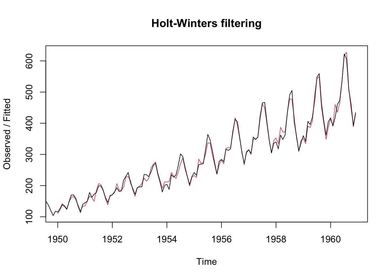
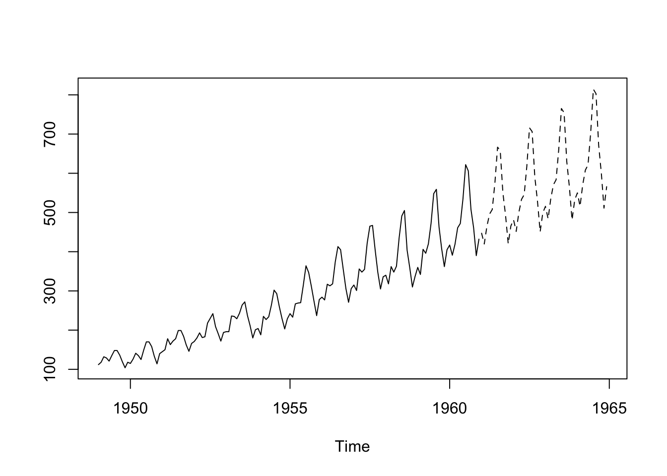
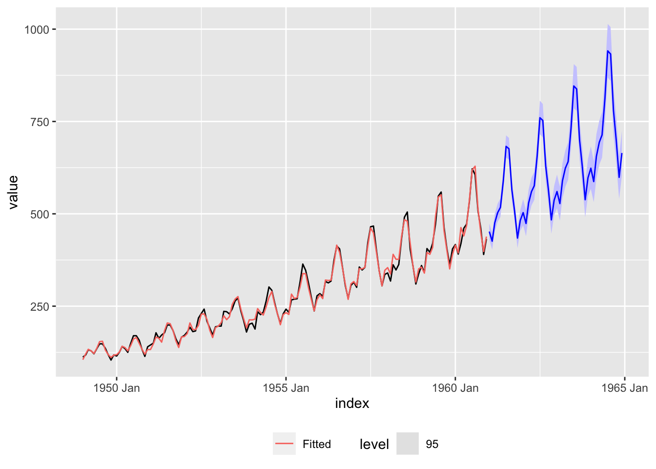
3.4.3 “Four-year-ahead forecasts” and “air passenger data” Modern Look
Book code
data (AirPassengers)<- AirPassengers<- HoltWinters (AP, seasonal = "mult" )plot (AP.hw)
Tidyverts code
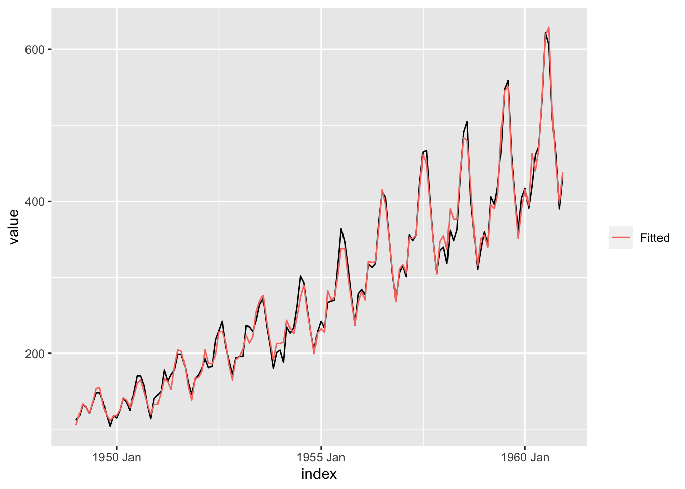
data (AirPassengers)<- as_tsibble (AirPassengers) |> mutate (Year = year (index),Month = month (index)<- ap |> model (Multiplicative = ETS (value ~ trend ("M" ) + error ("A" ) + season ("M" ),opt_crit = "amse" , nmse = 1 ))augment (ap_hw) |> ggplot (aes (x = index, y = value)) + geom_line () + geom_line (aes (y = .fitted, color = "Fitted" )) + labs (color = "" )
<- predict (AP.hw, n.ahead = 4 * 12 )ts.plot (AP, AP.predict, lty = 1 : 2 )
|> forecast (h = "4 years" ) |> autoplot (ap, level = 95 ) + geom_line (aes (y = .fitted, color = "Fitted" ),data = augment (ap_hw)) + scale_color_discrete (name = "" ) + theme (legend.position = "bottom" )
Show the Book code in full
data (AirPassengers)<- AirPassengers<- HoltWinters (AP, seasonal = "mult" )plot (AP.hw)<- predict (AP.hw, n.ahead = 4 * 12 )ts.plot (AP, AP.predict, lty = 1 : 2 )
Show the Tidyverts code in full
data (AirPassengers)<- as_tsibble (AirPassengers) |> mutate (Year = year (index),Month = month (index)<- ap |> model (Multiplicative = ETS (value ~ trend ("M" ) + error ("A" ) + season ("M" ),opt_crit = "amse" , nmse = 1 ))augment (ap_hw) |> ggplot (aes (x = index, y = value)) + geom_line () + geom_line (aes (y = .fitted, color = "Fitted" )) + labs (color = "" )|> forecast (h = "4 years" ) |> autoplot (ap, level = 95 ) + geom_line (aes (y = .fitted, color = "Fitted" ),data = augment (ap_hw)) + scale_color_discrete (name = "" )
3.5 Summary of Modern R commands used in examples