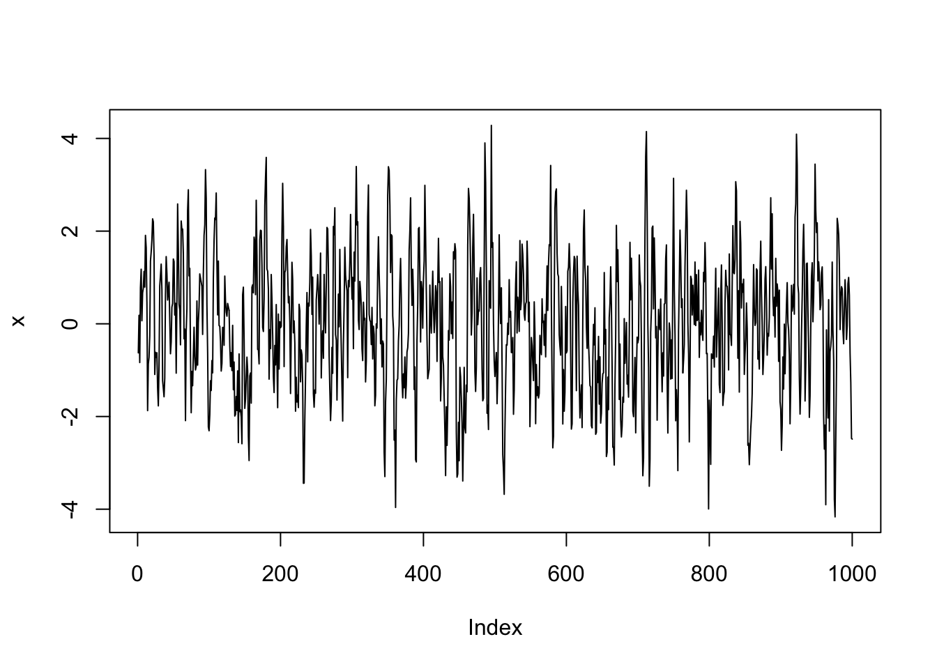
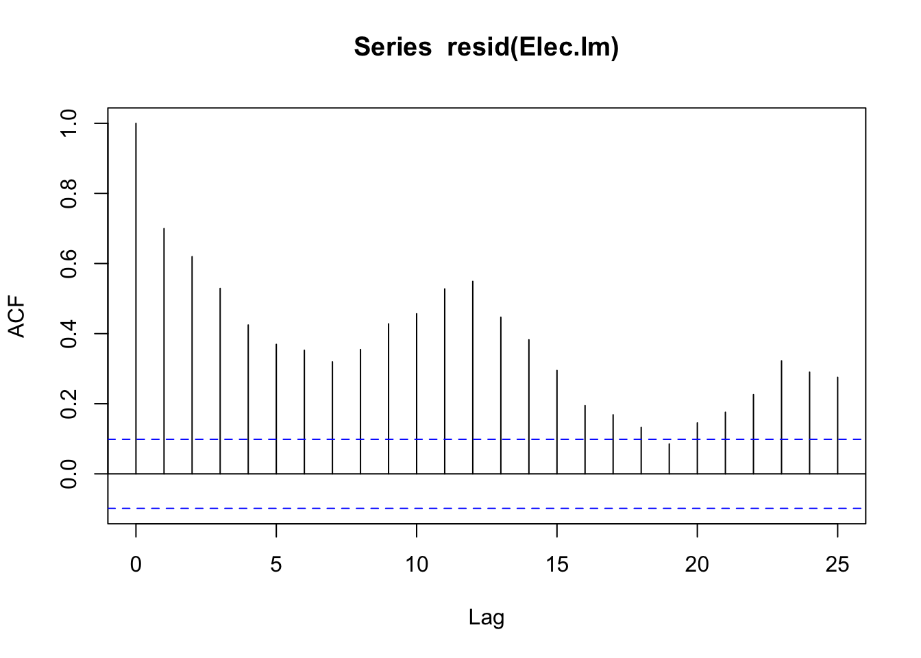
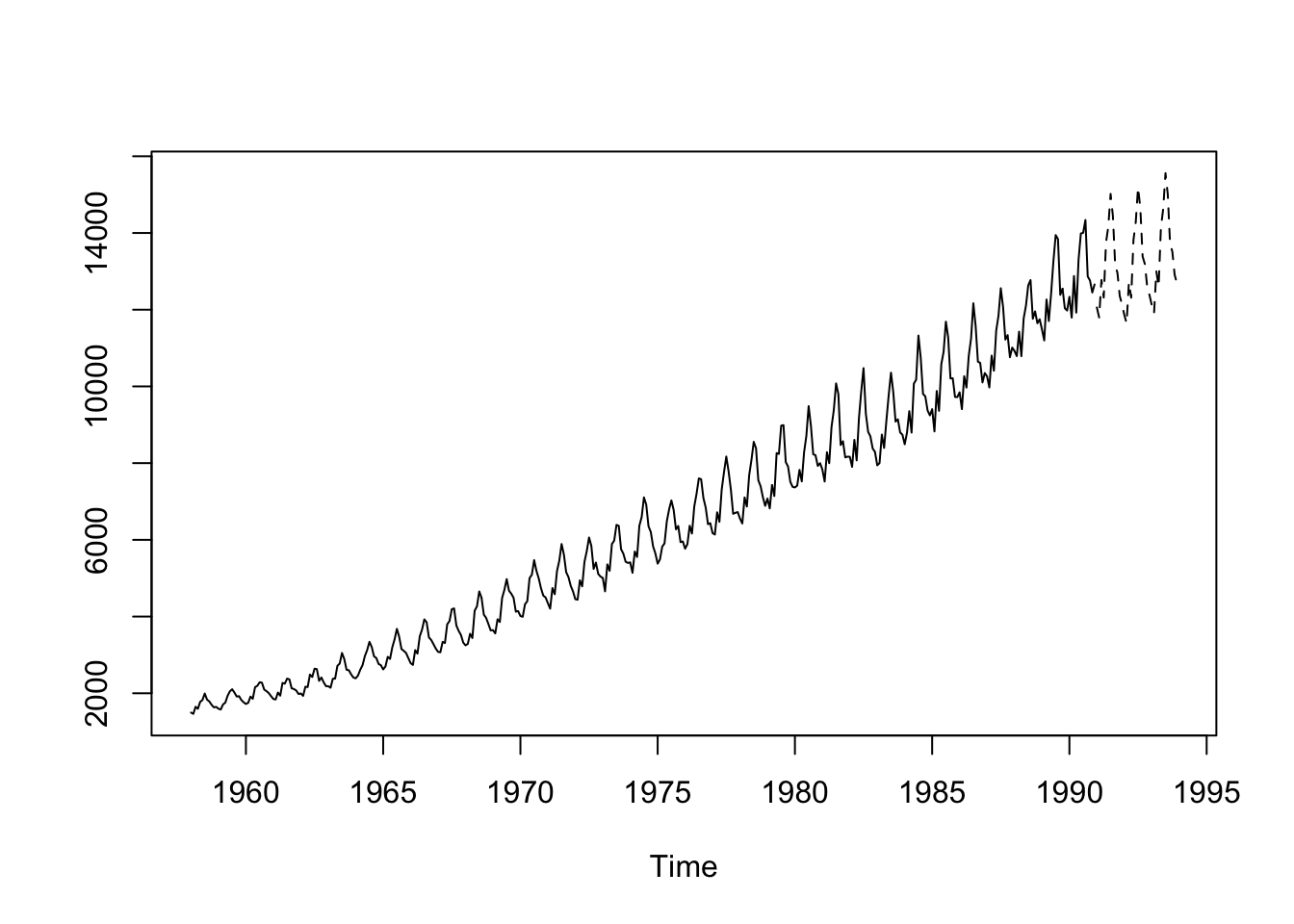
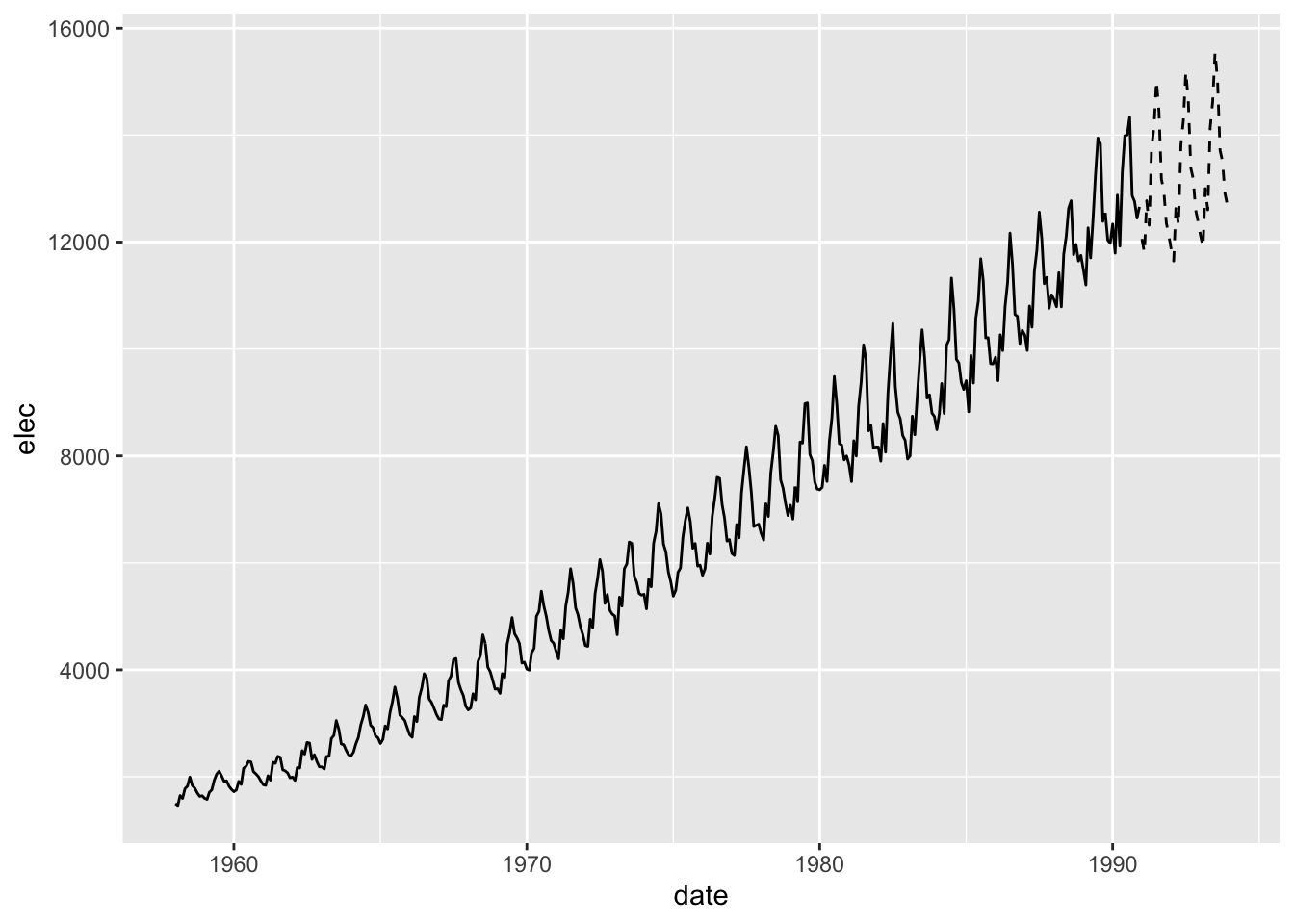
In this chapter, we consider stationary models that may be suitable for residual series that contain no obvious trends or seasonal cycles. The fitted stationary models may then be combined with the fitted regression model to improve forecasts.
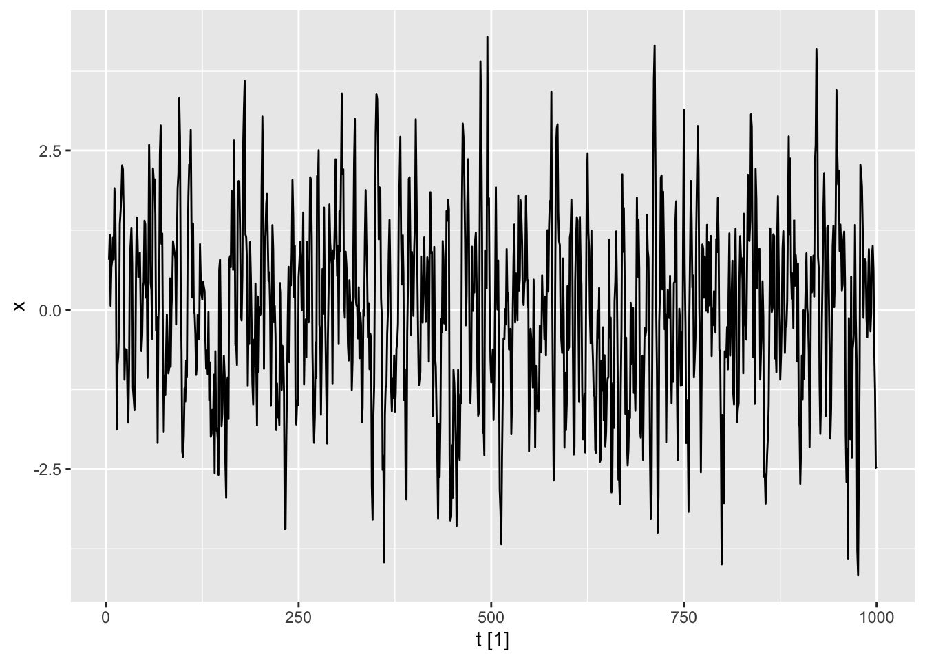
6.3.2 “R examples: Correlogram and simulation” Modern Look
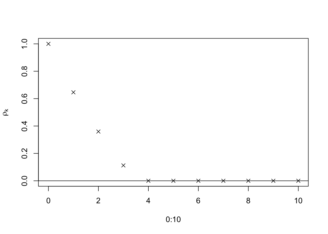
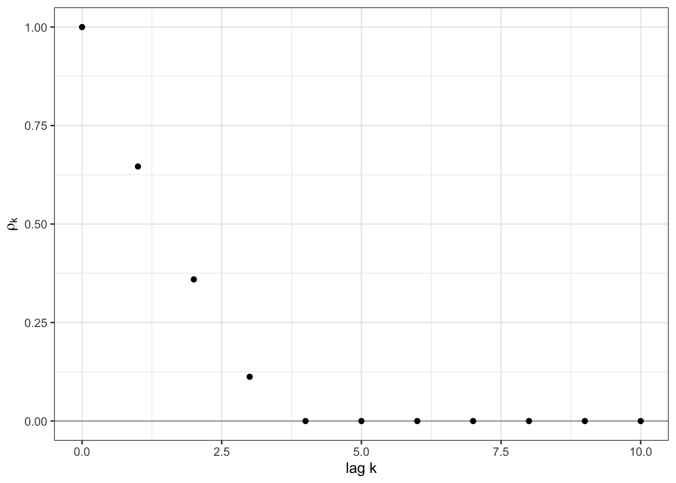
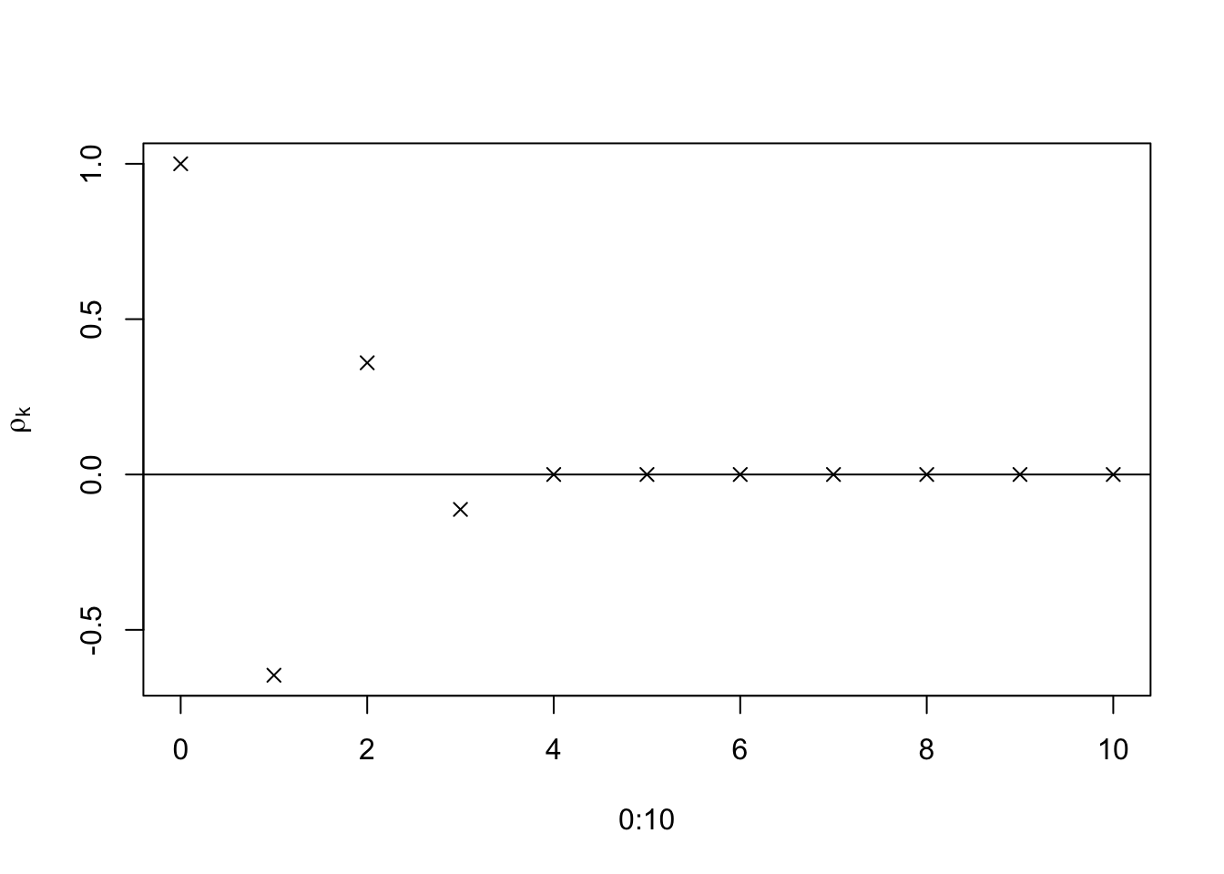
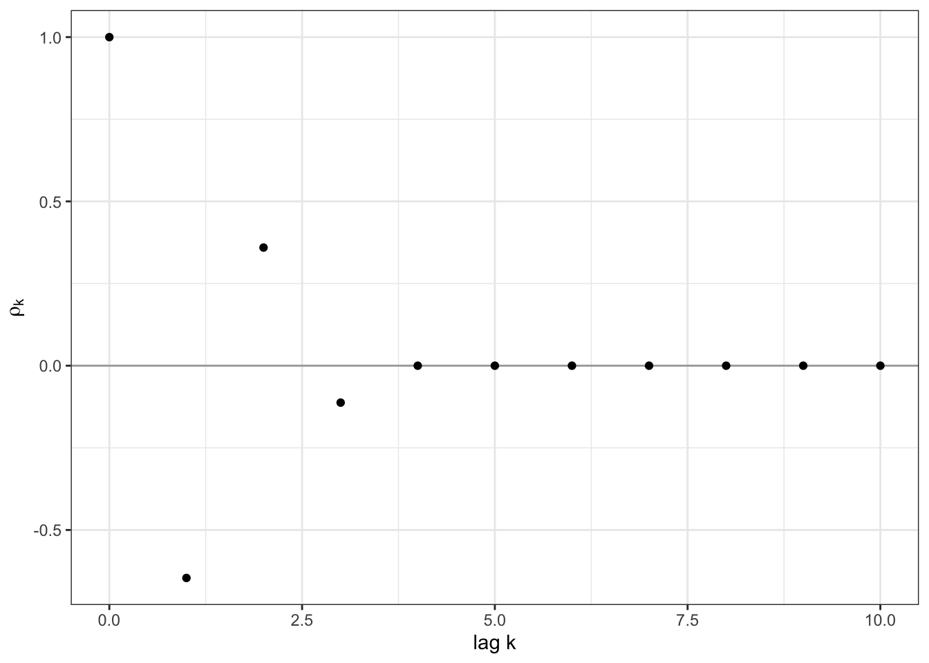
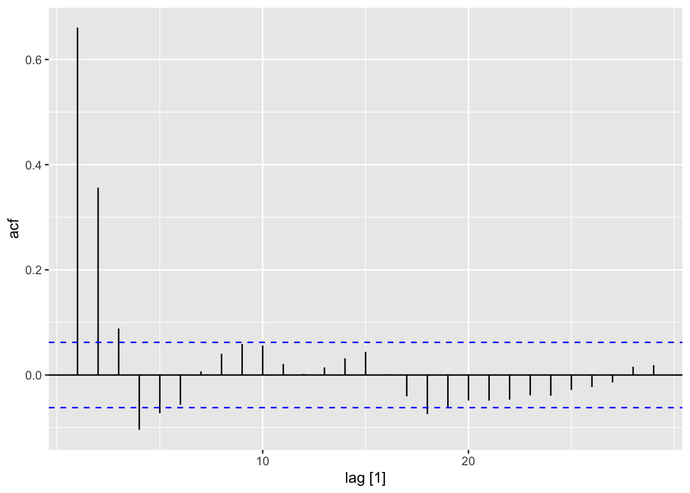
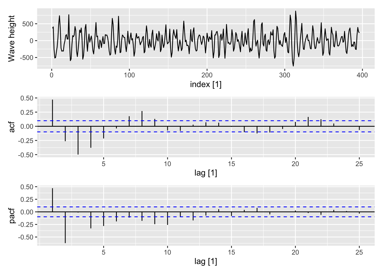
dat |>ggplot(aes(x = order, y = rho.k2)) +geom_hline(yintercept =0, color ="darkgrey") +geom_point() +labs(y =expression(rho[k]), x ="lag k") +theme_bw()
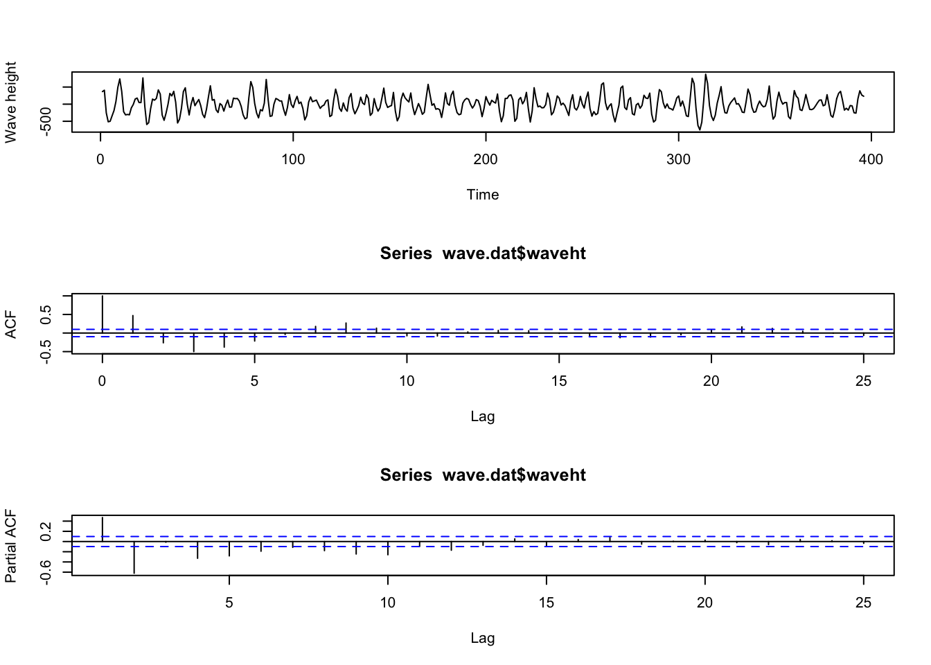
feasts::PACF(): Function PACF computes an estimate of the partial autocorrelation function of a (possibly multivariate) tsibble.
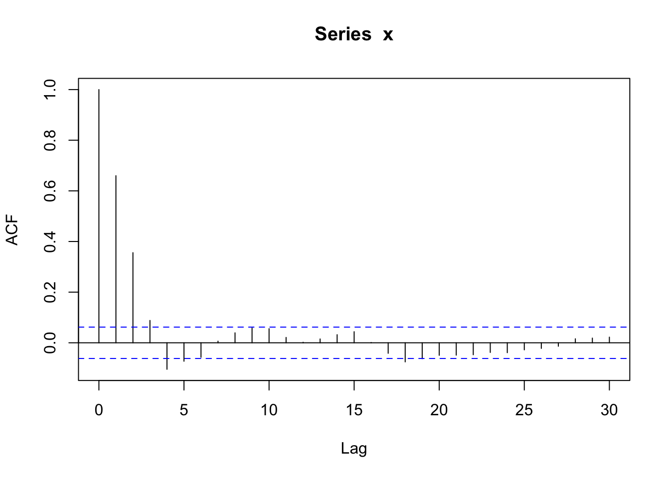
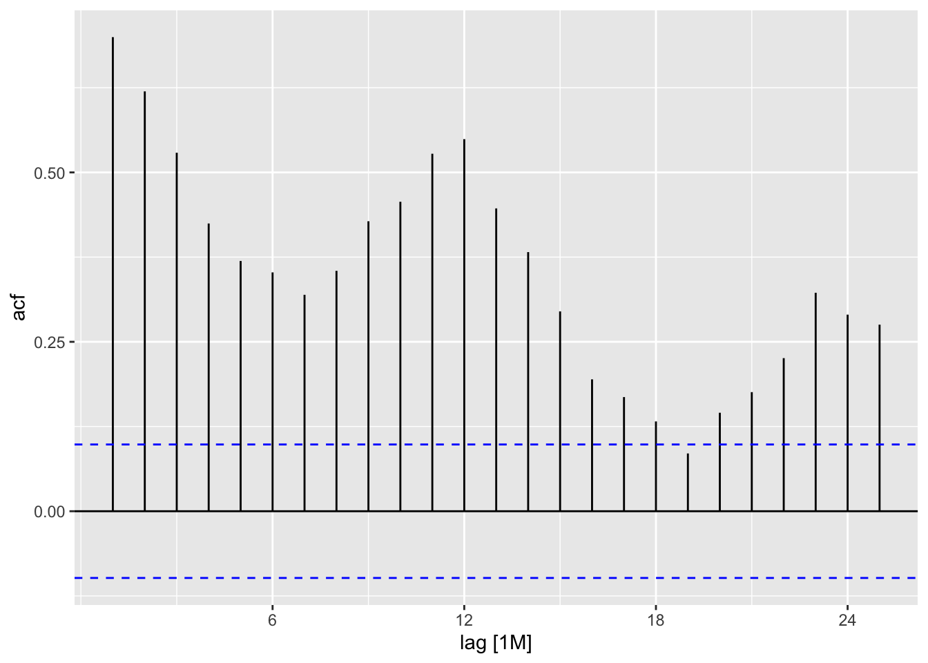
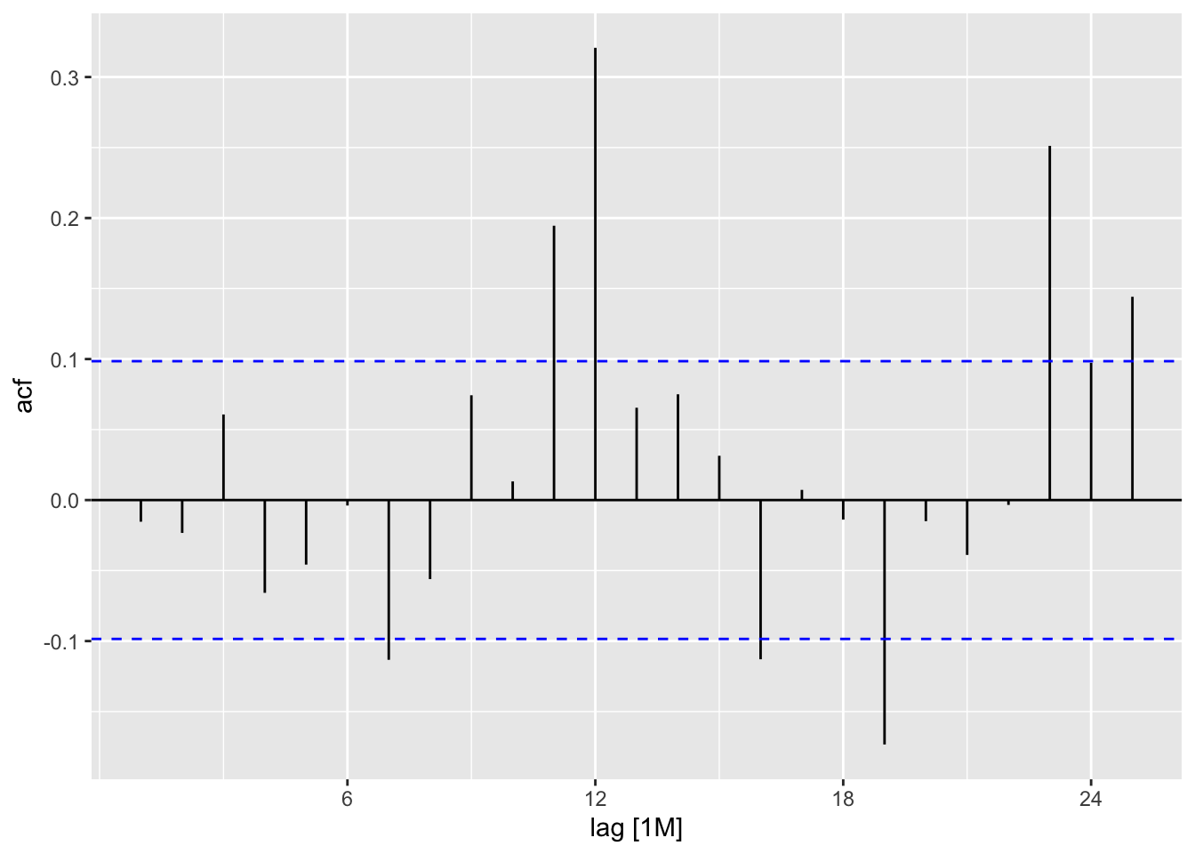
feasts::ACF(): The function ACF computes an estimate of the autocorrelation function of a (possibly multivariate) tsibble.
purrr:map2_dbl(): The map functions transform their input by applying a function to each element of a list or atomic vector and returning an object of the same length as the input.
ggplot2:geom_hline(): These geoms add reference lines (sometimes called rules) to a plot
base::expression(): If the text argument to one of the text-drawing functions in R is an expression, the argument is interpreted as a mathematical expression and the output will be formatted according to TeX-like rules.
slider::slide(): iterates through .x using a sliding window, applying .f to each sub-window of .x.
base::rev(): provides a reversed version of its argument.
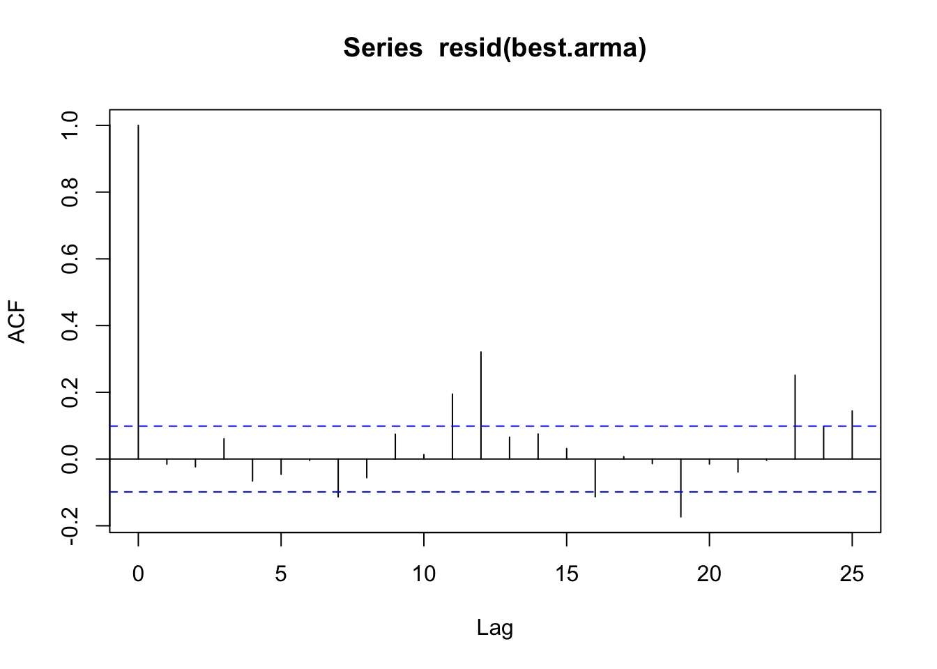
fable::ARIMA(): Searches through the model space specified in the specials to identify the best ARIMA model, with the lowest AIC, AICc or BIC value.
pdq(): The pdq special is used to specify non-seasonal components of the model.
PDQ(): The PDQ special is used to specify seasonal components of the model. To force a non-seasonal fit, specify PDQ(0, 0, 0) in the RHS of the model formula.