Chapter 5: Regression

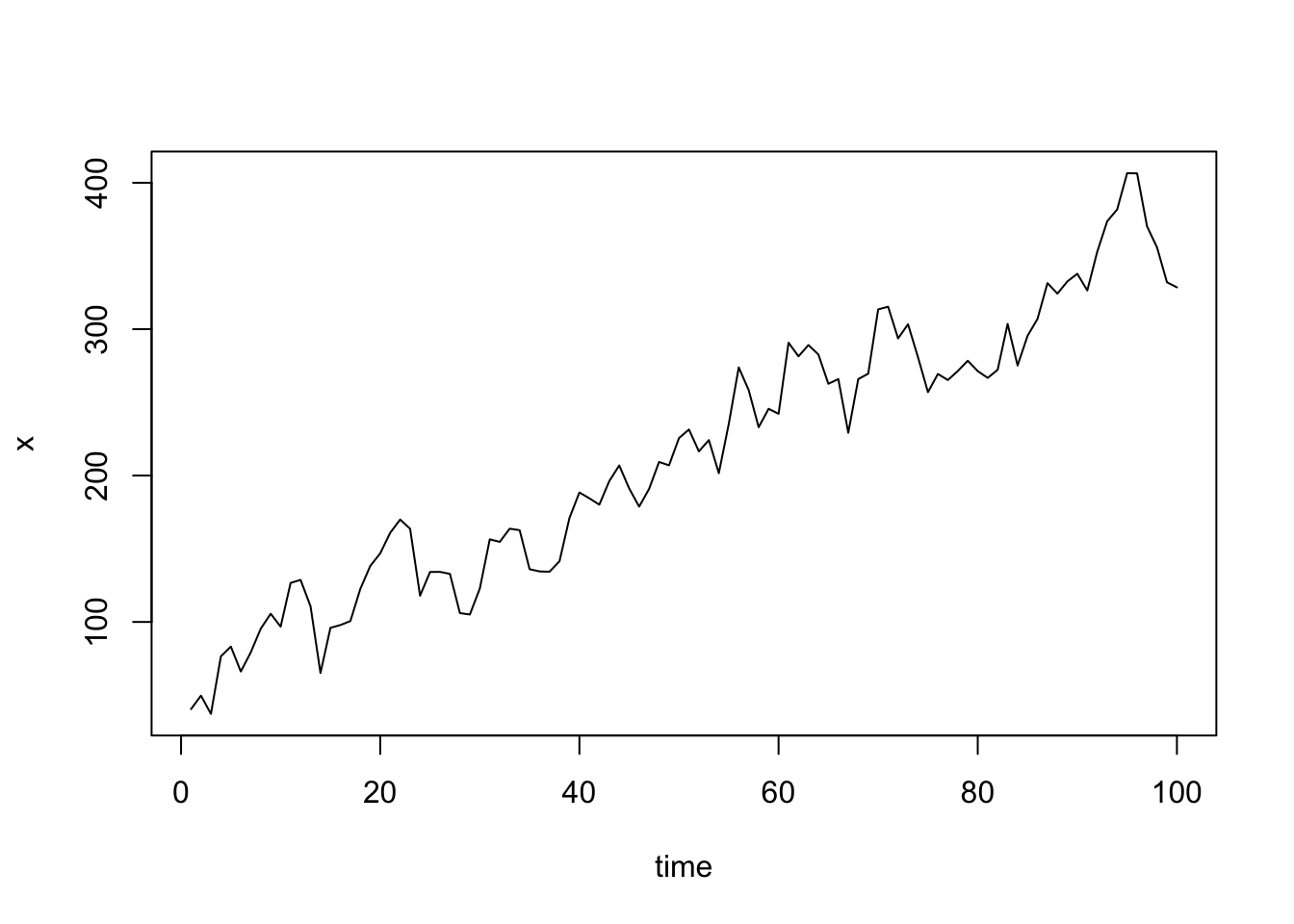
In this chapter various regression models are studied that are suitable for a time series analysis of data that contain deterministic trends and regular seasonal changes. We begin by looking at linear models for trends and then introduce regression models that account for seasonal variation using indicator and harmonic variables. Regression models can also include explanatory variables. The logarithmic transformation, which is often used to stabilise the variance, is also considered.

Note: The difference in the base R AIC() function and the AIC calculation in the Tidyverts output is a matter of constant terms. The general notion of reducing the value of AIC with your model still holds.

5.2.3 “Simulation in `R`” Modern Look

Book code

set.seed(1)
z <- w <- rnorm(100, sd = 20)
for (t in 2:100) z[t] <- 0.8 * z[t - 1] + w[t]
Time <- 1:100
x <- 50 + 3 * Time + z
plot(x, xlab = "time", type = "l")

Tidyverts code

pacman::p_load("tsibble", "fable", "feasts",
    "tsibbledata", "fable.prophet", "tidyverse",
    "patchwork")

set.seed(1)

dat <- tibble(w = rnorm(100, sd = 20)) |>
    mutate(
        Time = 1:n(),
         z = purrr::accumulate2(
            lag(w), w, 
            \(acc, nxt, w) 0.8 * acc + w,
            .init = 0)[-1],
          x = 50 + 3 * Time + z
            ) |>
    tsibble::as_tsibble(index = Time)
autoplot(dat, .var = x)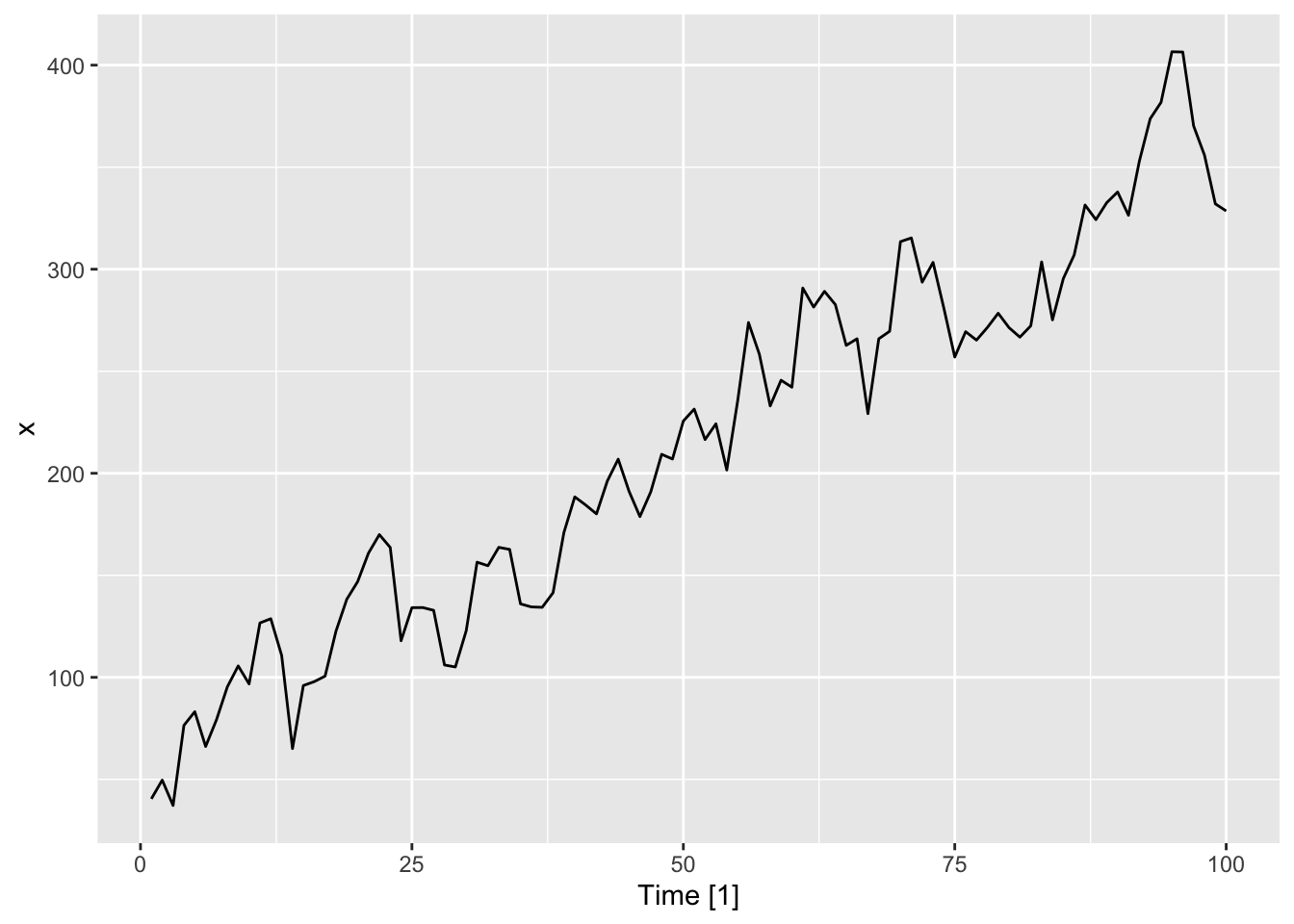

Show the Book code in full

set.seed(1)
z <- w <- rnorm(100, sd = 20)
for (t in 2:100) z[t] <- 0.8 * z[t - 1] + w[t]
Time <- 1:100
x <- 50 + 3 * Time + z
plot(x, xlab = "time", type = "l")

Show the Tidyverts code in full

pacman::p_load("tsibble", "fable", "feasts",
    "tsibbledata", "fable.prophet", "tidyverse", "patchwork")

set.seed(1)

dat <- tibble(w = rnorm(100, sd = 20)) |>
    mutate(
        Time = 1:n(),
         z = purrr::accumulate2(
            lag(w), w, 
            \(acc, nxt, w) 0.8 * acc + w,
            .init = 0)[-1],
          x = 50 + 3 * Time + z
            ) |>
    tsibble::as_tsibble(index = Time)
autoplot(dat, .var = x)

5.3.1 “Model fitted to simulated data” Modern Look

Book code

x.lm <- lm(x ~ Time)
coef(x.lm)

(Intercept)        Time 
  58.551218    3.063275

Tidyverts code

dat_lm <- dat |>
  model(lm = TSLM(x ~ Time))
tidy(dat_lm) |> pull(estimate)

[1] 58.551218  3.063275

sqrt(diag(vcov(x.lm)))

(Intercept)        Time 
 4.88006278  0.08389621

tidy(dat_lm) |> pull(std.error)

[1] 4.88006278 0.08389621

acf(resid(x.lm))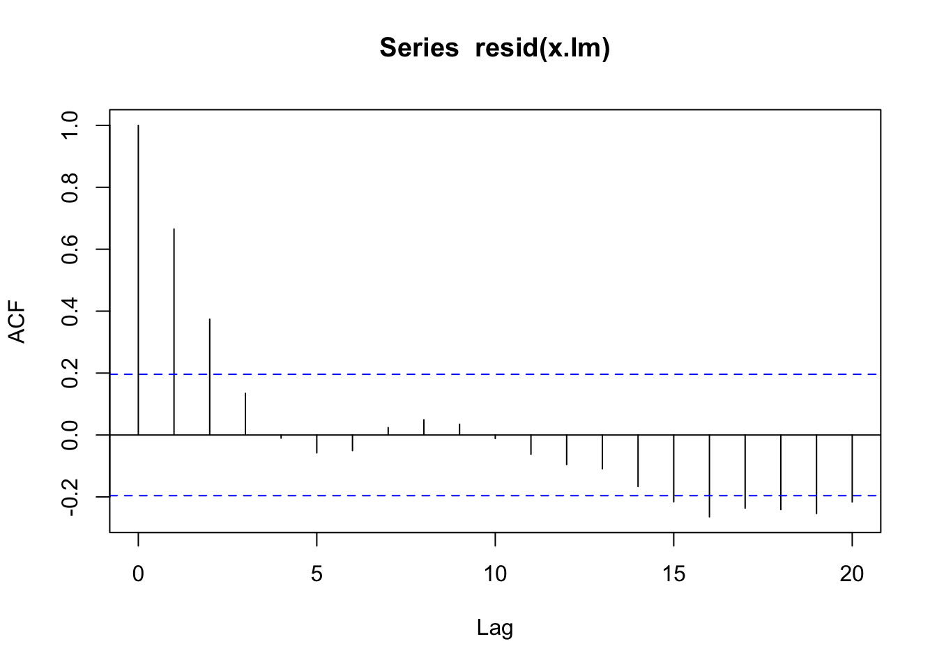

residuals(dat_lm) |> feasts::ACF(var = .resid) |> autoplot()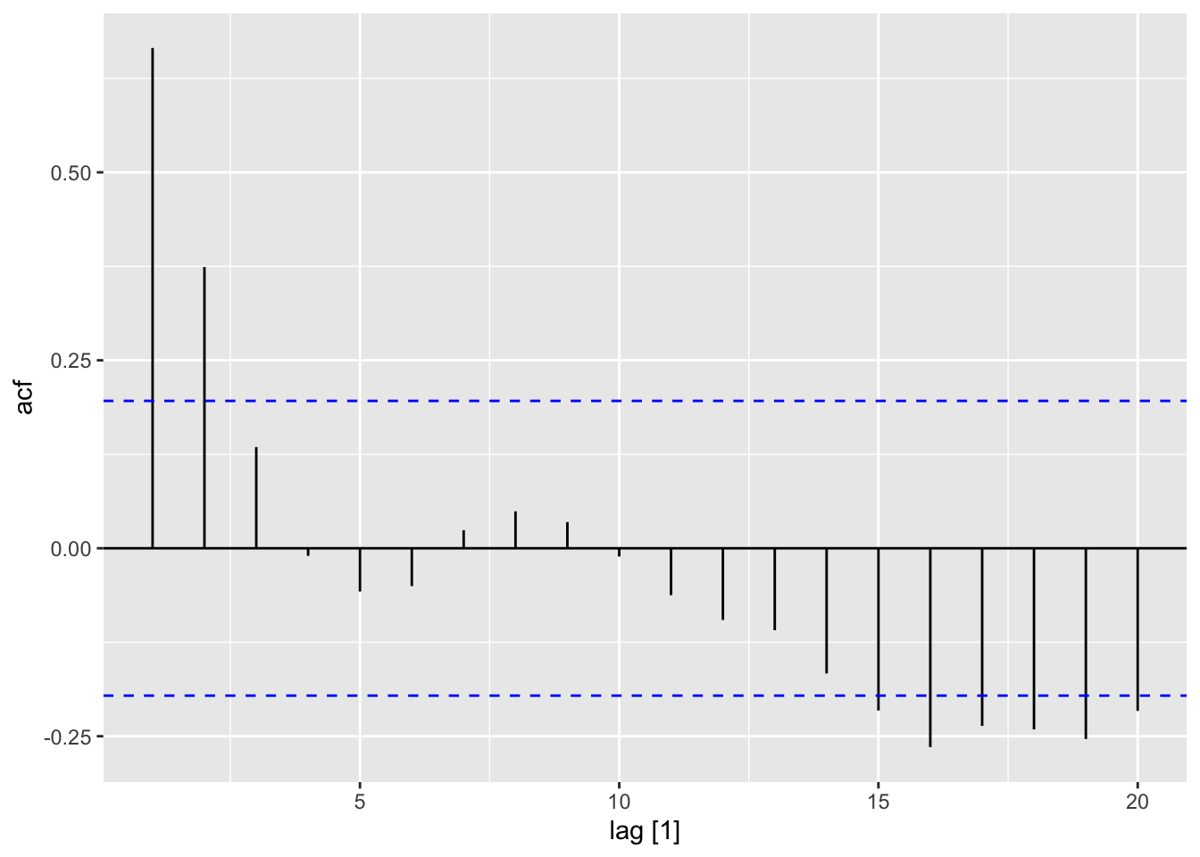

pacf(resid(x.lm))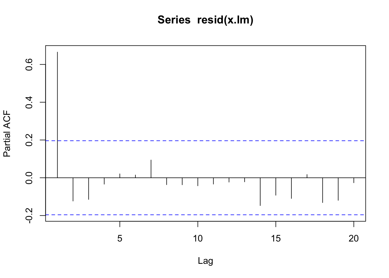

residuals(dat_lm) |> PACF(var = .resid) |> autoplot()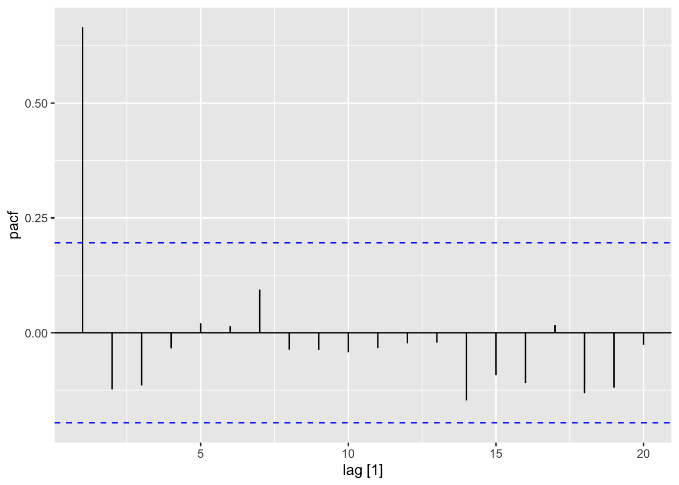

Show the Book code in full

x.lm <- lm(x ~ Time)
coef(x.lm)
sqrt(diag(vcov(x.lm)))
acf(resid(x.lm))
pacf(resid(x.lm))

Show the Tidyverts code in full

dat_lm <- dat |>
  model(lm = TSLM(x ~ Time))
tidy(dat_lm) |> pull(estimate)
tidy(dat_lm) |> pull(std.error)
residuals(dat_lm) |> feasts::ACF(var = .resid) |> autoplot()
residuals(dat_lm) |> feasts::PACF(var = .resid) |> autoplot()

5.3.1 “Model fitted to the temperature series (1970-2005)” Modern Look

Book code

Global <- scan("data/global.dat")
Global.ts <- ts(Global, st = c(1856, 1), end = c(2005, 12), fr = 12)
temp <- window(Global.ts, start = 1970)
temp.lm <- lm(temp ~ time(temp))
coef(temp.lm)

(Intercept)  time(temp) 
 -34.920409    0.017654

Tidyverts code

global <- tibble(x = scan("data/global.dat")) |>
    mutate(
        date = seq(
            ymd("1856-01-01"),
            by = "1 months",
            length.out = n()),
        year = year(date),
        year_month = tsibble::yearmonth(date),
        stats_time = year + c(0:11)/12)

global_ts <- global |>
    as_tsibble(index = year_month)

temp_tidy <- global_ts |> filter(year >= 1970)
temp_lm <- temp_tidy |>
  model(lm = TSLM(x ~ stats_time ))
tidy(temp_lm) |> pull(estimate)

[1] -34.920409   0.017654

confint(temp.lm)

                   2.5 %       97.5 %
(Intercept) -37.21001248 -32.63080554
time(temp)    0.01650228   0.01880572

tidy(temp_lm) |>
  mutate(
    `2.5%` = estimate + qnorm(.025) * std.error,
    `97.5%` = estimate + qnorm(.975) * std.error
  )

# A tibble: 2 × 8
  .model term        estimate std.error statistic   p.value   `2.5%`  `97.5%`
  <chr>  <chr>          <dbl>     <dbl>     <dbl>     <dbl>    <dbl>    <dbl>
1 lm     (Intercept) -34.9     1.16         -30.0 2.15e-107 -37.2    -32.6   
2 lm     stats_time    0.0177  0.000586      30.1 4.99e-108   0.0165   0.0188

acf(resid(lm(temp ~ time(temp))))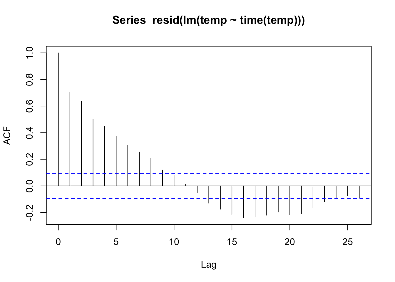

residuals(temp_lm) |>
  feasts::ACF(var = .resid) |>
  autoplot()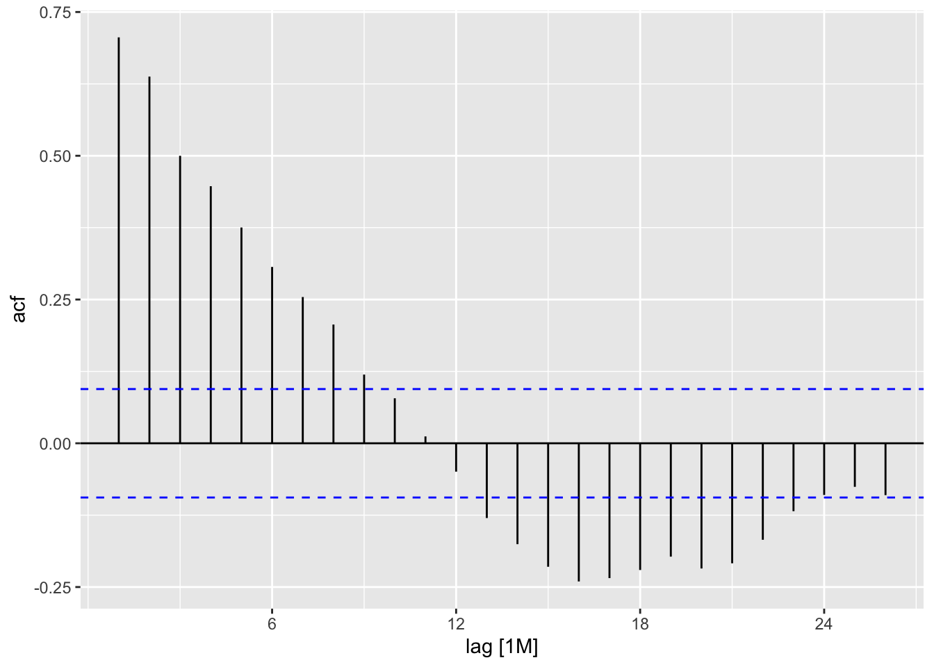

Show the Book code in full

Global <- scan("data/global.dat")
Global.ts <- ts(Global, st = c(1856, 1), end = c(2005, 12), fr = 12)
temp <- window(Global.ts, start = 1970)
temp.lm <- lm(temp ~ time(temp))
coef(temp.lm)
confint(temp.lm)
acf(resid(lm(temp ~ time(temp))))

Show the Tidyverts code in full

global <- tibble(x = scan("data/global.dat")) |>
    mutate(
        date = seq(
            ymd("1856-01-01"),
            by = "1 months",
            length.out = n()),
        year = year(date),
        year_month = tsibble::yearmonth(date),
        stats_time = year + c(0:11)/12)

global_ts <- global |>
    as_tsibble(index = year_month)

temp_tidy <- global_ts |> filter(year >= 1970)
temp_lm <- temp_tidy |>
  model(lm = TSLM(x ~ stats_time ))
tidy(temp_lm) |> pull(estimate)

tidy(temp_lm) |>
  mutate(
    `2.5%` = estimate + qnorm(.025) * std.error,
    `97.5%` = estimate + qnorm(.975) * std.error
  )

residuals(temp_lm) |>
  feasts::ACF(var = .resid) |>
  autoplot()

5.4.1 “GLS fit to simulated series” Modern Look

Book code

library(nlme)
x.gls <- gls(x ~ Time, cor = corAR1(0.8))
coef(x.gls)

(Intercept)        Time 
  58.233018    3.042245

Tidyverts code

pacman::p_load(tidymodels, multilevelmod,
  nlme, broom.mixed)
gls_spec <- linear_reg() |>
  set_engine("gls", correlation = nlme::corAR1(0.8))

dat_gls <- gls_spec |>
  fit(x ~ Time, data = dat)

broom.mixed::tidy(dat_gls) |>
  pull(estimate)

[1] 58.233018  3.042245

sqrt(diag(vcov(x.gls)))

(Intercept)        Time 
 11.9245679   0.2024447

broom.mixed::tidy(dat_gls) |>
  pull(std.error)

[1] 11.9245679  0.2024447

Show the Book code in full

library(nlme)
x.gls <- gls(x ~ Time, cor = corAR1(0.8))
coef(x.gls)
sqrt(diag(vcov(x.gls)))

Show the Tidyverts code in full

pacman::p_load(tidymodels, multilevelmod, nlme, broom.mixed)
gls_spec <- linear_reg() |>
  set_engine("gls", correlation = nlme::corAR1(0.8))

dat_gls <- gls_spec |>
  fit(x ~ Time, data = dat)

broom.mixed::tidy(dat_gls) |>
  pull(estimate)

broom.mixed::tidy(dat_gls) |>
  pull(std.error)

5.4.2 “Confidence interval for the trend in the temperature series” Modern Look

Book code

temp.gls <- gls(temp ~ time(temp), cor = corAR1(0.7))
confint(temp.gls)

                   2.5 %       97.5 %
(Intercept) -39.80571502 -28.49659113
time(temp)    0.01442275   0.02011148

Tidyverts code

temp_spec <- linear_reg() |>
  set_engine("gls", correlation = nlme::corAR1(0.7))

temp_gls <- temp_spec |>
  fit(x ~ stats_time, data = temp_tidy)

tidy(temp_gls) |>
  mutate(
    `2.5%` = estimate + qnorm(.025) * std.error,
    `97.5%` = estimate + qnorm(.975) * std.error
  )

# A tibble: 2 × 7
  term        estimate std.error statistic  p.value   `2.5%`  `97.5%`
  <chr>          <dbl>     <dbl>     <dbl>    <dbl>    <dbl>    <dbl>
1 (Intercept) -34.2      2.89        -11.8 3.54e-28 -39.8    -28.5   
2 stats_time    0.0173   0.00145      11.9 2.05e-28   0.0144   0.0201

Show the Book code in full

temp.gls <- gls(temp ~ time(temp), cor = corAR1(0.7))
confint(temp.gls)

Show the Tidyverts code in full

temp_spec <- linear_reg() |>
  set_engine("gls", correlation = nlme::corAR1(0.7))

temp_gls <- temp_spec |>
  fit(x ~ stats_time, data = temp)

tidy(temp_gls) |>
  mutate(
    `2.5%` = estimate + qnorm(.025) * std.error,
    `97.5%` = estimate + qnorm(.975) * std.error
  )

5.5.3 “Example: Seasonal model for the temperature series” Modern Look

Book code

Seas <- cycle(temp)
Time <- time(temp)
temp.lm <- lm(temp ~ 0 + Time + factor(Seas))
coef(temp.lm)

          Time  factor(Seas)1  factor(Seas)2  factor(Seas)3  factor(Seas)4 
    0.01770758   -34.99726483   -34.98801824   -35.01002165   -35.01227506 
 factor(Seas)5  factor(Seas)6  factor(Seas)7  factor(Seas)8  factor(Seas)9 
  -35.03369513   -35.02505965   -35.02689640   -35.02476092   -35.03831988 
factor(Seas)10 factor(Seas)11 factor(Seas)12 
  -35.05248996   -35.06557670   -35.04871900

Tidyverts code

temp_tidy <- temp_tidy |>
  mutate(month = factor(month(date)))
temp_lm <- temp_tidy |>
  model(TSLM(x ~ 0 + stats_time + month))

temp_lm |>
  tidy() |>
  pull(estimate)

 [1]   0.01770758 -34.99726483 -34.98801824 -35.01002165 -35.01227506
 [6] -35.03369513 -35.02505965 -35.02689640 -35.02476092 -35.03831988
[11] -35.05248996 -35.06557670 -35.04871900

new.t <- seq(2006, len = 2 * 12, by = 1/12)
alpha <- coef(temp.lm)[1]
beta <- rep(coef(temp.lm)[2:13], 2)
(alpha * new.t + beta)[1:4]

factor(Seas)1 factor(Seas)2 factor(Seas)3 factor(Seas)4 
    0.5241458     0.5348681     0.5143403     0.5135625

new_dat <- tibble(
  stats_time = c(2006 + c(0:11)/12, 2007 + c(0:11)/12),
  month = factor(rep(1:12, 2)),
  alpha = tidy(temp_lm) |> slice(1) |> pull(estimate),
  beta = rep(tidy(temp_lm) |> slice(2:13) |> pull(estimate), 2))

new_dat |>
  mutate(estimate = alpha * stats_time + beta) |>
  slice(1:4)

# A tibble: 4 × 5
  stats_time month  alpha  beta estimate
       <dbl> <fct>  <dbl> <dbl>    <dbl>
1      2006  1     0.0177 -35.0    0.524
2      2006. 2     0.0177 -35.0    0.535
3      2006. 3     0.0177 -35.0    0.514
4      2006. 4     0.0177 -35.0    0.514

new.dat <- data.frame(Time = new.t, Seas = rep(1:12, 2))
predict(temp.lm, new.dat)[1:24]

        1         2         3         4         5         6         7         8 
0.5241458 0.5348681 0.5143403 0.5135625 0.4936181 0.5037292 0.5033681 0.5069792 
        9        10        11        12        13        14        15        16 
0.4948958 0.4822014 0.4705903 0.4889236 0.5418534 0.5525756 0.5320479 0.5312701 
       17        18        19        20        21        22        23        24 
0.5113256 0.5214367 0.5210756 0.5246867 0.5126034 0.4999090 0.4882979 0.5066312

temp_lm |>
  forecast(new_data=as_tsibble(new_dat, index = stats_time)) |>
  pull(.mean)

 [1] 0.5241458 0.5348681 0.5143403 0.5135625 0.4936181 0.5037292 0.5033681
 [8] 0.5069792 0.4948958 0.4822014 0.4705903 0.4889236 0.5418534 0.5525756
[15] 0.5320479 0.5312701 0.5113256 0.5214367 0.5210756 0.5246867 0.5126034
[22] 0.4999090 0.4882979 0.5066312

Show the Book code in full

Seas <- cycle(temp)
Time <- time(temp)
temp.lm <- lm(temp ~ 0 + Time + factor(Seas))
coef(temp.lm)
new.t <- seq(2006, len = 2 * 12, by = 1/12)
alpha <- coef(temp.lm)[1]
beta <- rep(coef(temp.lm)[2:13], 2)
(alpha * new.t + beta)[1:4]
new.dat <- data.frame(Time = new.t, Seas = rep(1:12, 2))
predict(temp.lm, new.dat)[1:24]

Show the Tidyverts code in full

new_dat <- tibble(
  stats_time = c(2006 + c(0:11)/12, 2007 + c(0:11)/12),
  month = factor(rep(1:12, 2)),
  alpha = tidy(temp_lm) |> slice(1) |> pull(estimate),
  beta = rep(tidy(temp_lm) |> slice(2:13) |> pull(estimate), 2))

new_dat |>
  mutate(estimate = alpha * stats_time + beta) |>
  slice(1:4)

temp_lm |>
  forecast(new_data=as_tsibble(new_dat, index = stats_time)) |>
  pull(.mean)

5.6 “Harmonic seasonal models” Modern Look

Book code

TIME <- seq(1, 12, len = 1000)
plot(TIME, sin(2 * pi * TIME/12), type = "l")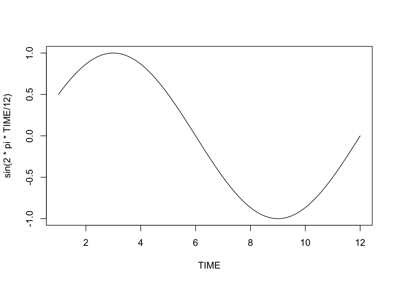

Tidyverts code

dat <- tibble(
  TIME = seq(1, 12, len = 1000),
  y1 = sin(2 * pi * TIME/12),
  y2 = sin(2 * pi * TIME/12) + 0.2 * sin(2 * pi * 2 *
      TIME/12) + 0.1 * sin(2 * pi * 4 * TIME/12) + 0.1 *
      cos(2 * pi * 4 * TIME/12))
ggplot(dat, aes(x = TIME, y = y1)) + geom_line()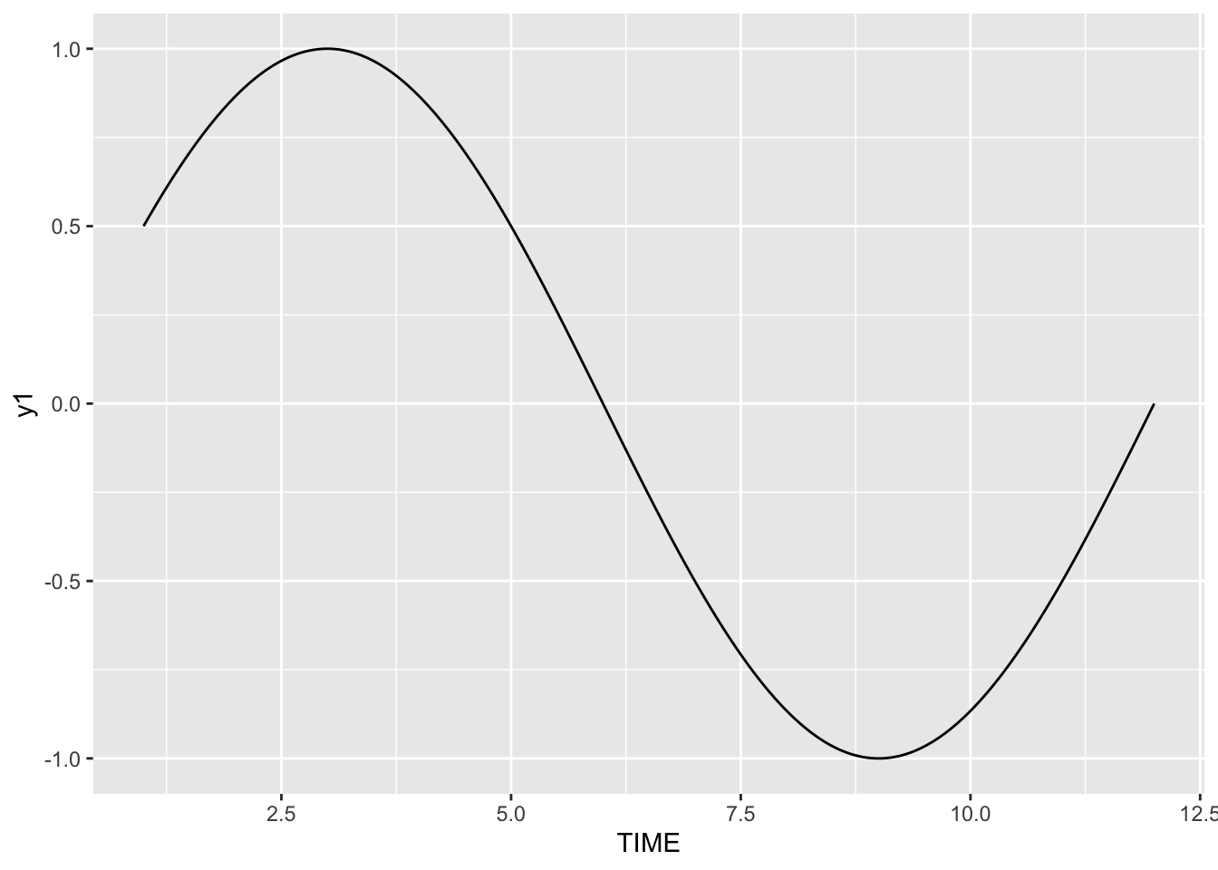

plot(TIME, sin(2 * pi * TIME/12) + 0.2 * sin(2 * pi * 2 *
      TIME/12) + 0.1 * sin(2 * pi * 4 * TIME/12) + 0.1 *
      cos(2 * pi * 4 * TIME/12), type = "l")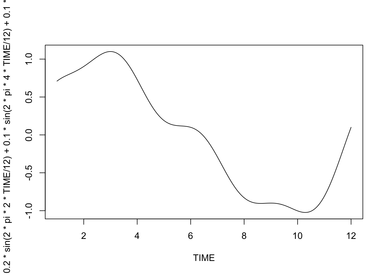

ggplot(dat, aes(x = TIME, y = y2)) + geom_line()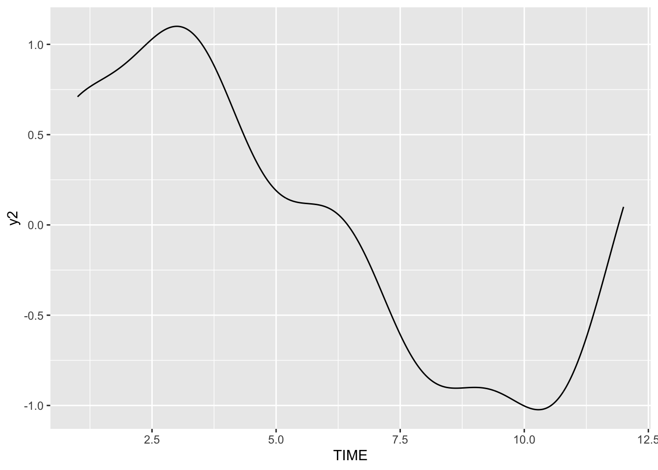

Show the Book code in full

TIME <- seq(1, 12, len = 1000)
plot(TIME, sin(2 * pi * TIME/12), type = "l")
plot(TIME, sin(2 * pi * TIME/12) + 0.2 * sin(2 * pi * 2 *
      TIME/12) + 0.1 * sin(2 * pi * 4 * TIME/12) + 0.1 *
      cos(2 * pi * 4 * TIME/12), type = "l")

Show the Tidyverts code in full

dat <- tibble(
  TIME = seq(1, 12, len = 1000),
  y1 = sin(2 * pi * TIME/12),
  y2 = sin(2 * pi * TIME/12) + 0.2 * sin(2 * pi * 2 *
      TIME/12) + 0.1 * sin(2 * pi * 4 * TIME/12) + 0.1 *
      cos(2 * pi * 4 * TIME/12))
ggplot(dat, aes(x = TIME, y = y1)) + geom_line()
ggplot(dat, aes(x = TIME, y = y2)) + geom_line()

5.6.1 “Simulation” Modern Look

Book code

set.seed(1)
TIME <- 1:(10 * 12)
w <- rnorm(10 * 12, sd = 0.5)
Trend <- 0.1 + 0.005 * TIME + 0.001 * TIME^2
Seasonal <- sin(2*pi*TIME/12) + 0.2*sin(2*pi*2*TIME/12) +
               0.1*sin(2*pi*4*TIME/12) + 0.1*cos(2*pi*4*TIME/12)
x <- Trend + Seasonal + w
plot(x, type = "l")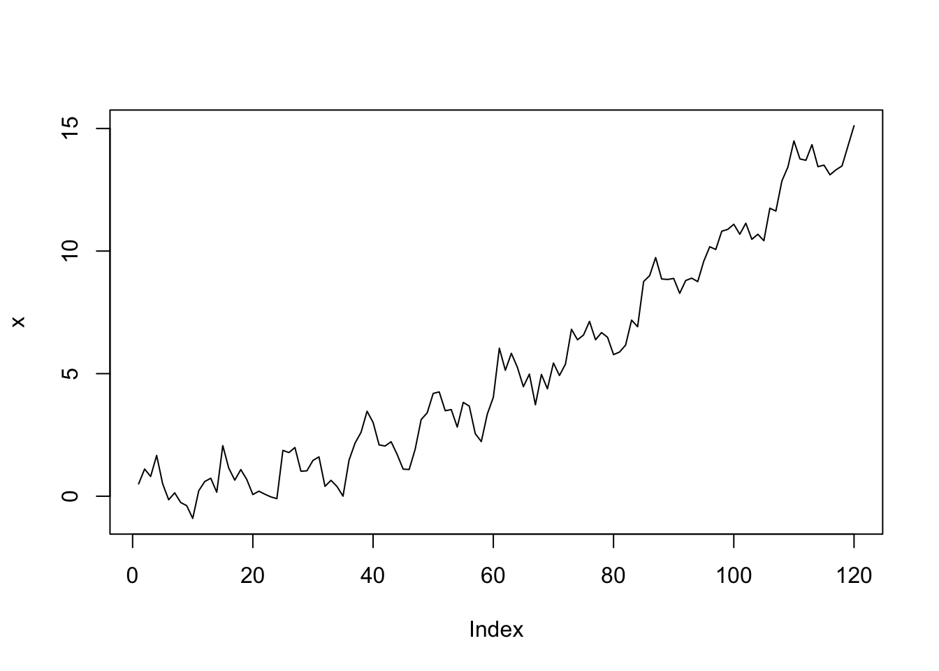

Tidyverts code

set.seed(1)
dat <- tibble(
  TIME = 1:(10 * 12),
  w = rnorm(10 * 12, sd = .5),
  trend = 0.1 + .005 * TIME + 0.001 * TIME^2,
  seasonal = sin(2 * pi * TIME / 12) +
    0.2 * sin(2 * pi * 2 * TIME / 12) +
    0.1 * sin(2 * pi * 4 * TIME / 12) +
    0.1 * cos(2 * pi * 4 * TIME / 12),
  x = trend + seasonal + w
)

ggplot(dat, aes(y = x, x = TIME)) + geom_line()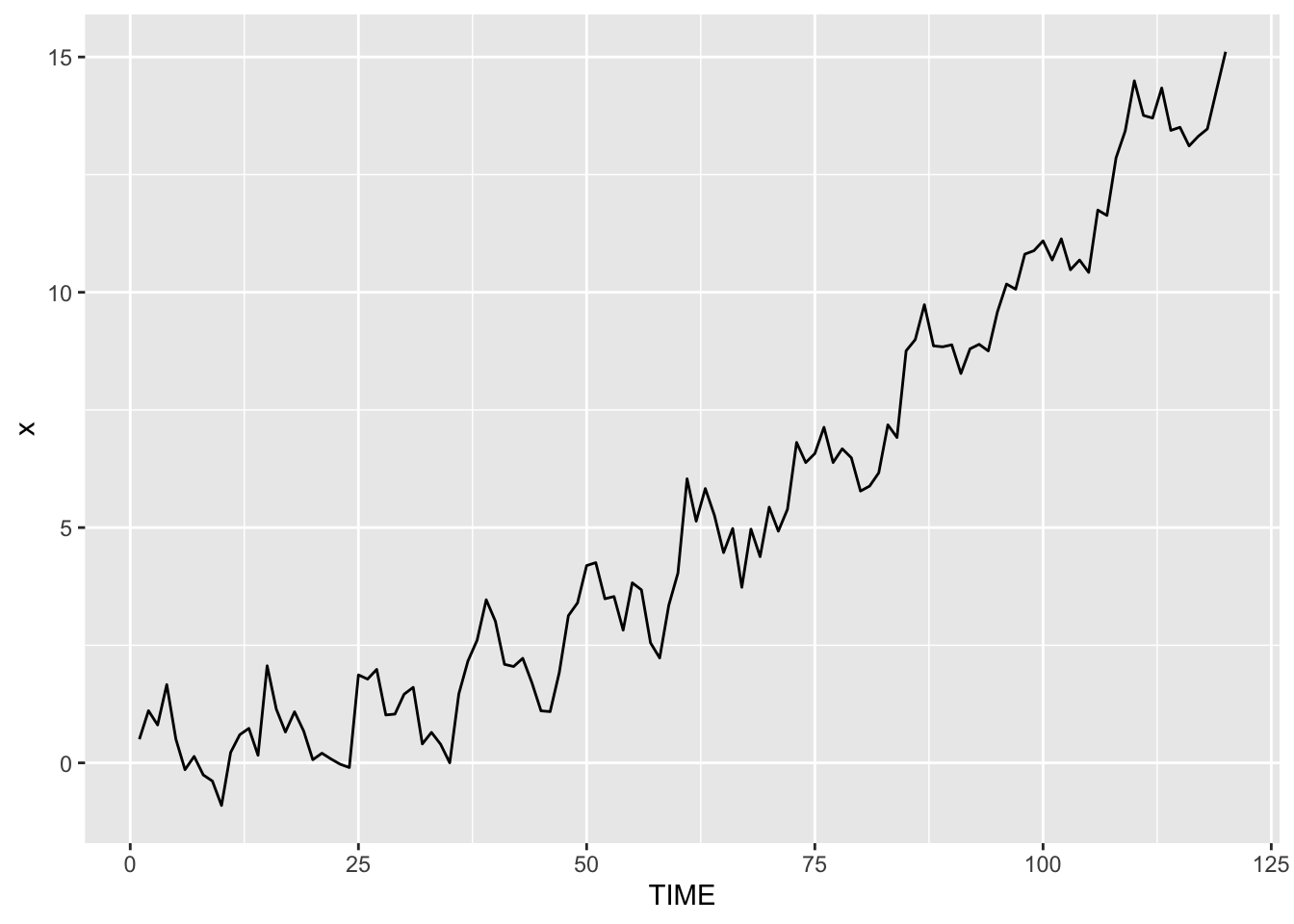

Show the Book code in full

set.seed(1)
TIME <- 1:(10 * 12)
w <- rnorm(10 * 12, sd = 0.5)
Trend <- 0.1 + 0.005 * TIME + 0.001 * TIME^2
Seasonal <- sin(2 * pi * TIME / 12) +
  0.2 * sin(2 * pi * 2 * TIME / 12) +
  0.1 * sin(2 * pi * 4 * TIME / 12) +
  0.1 * cos(2 * pi * 4 * TIME / 12)
x <- Trend + Seasonal + w
plot(x, type = "l")

Show the Tidyverts code in full

set.seed(1)
dat <- tibble(
  TIME = 1:(10 * 12),
  w = rnorm(10 * 12, sd = .5),
  trend = 0.1 + .005 * TIME + 0.001 * TIME^2,
  seasonal = sin(2 * pi * TIME / 12) +
    0.2 * sin(2 * pi * 2 * TIME / 12) +
    0.1 * sin(2 * pi * 4 * TIME / 12) +
    0.1 * cos(2 * pi * 4 * TIME / 12),
  x = trend + seasonal + w
)

ggplot(dat, aes(y = x, x = TIME)) + geom_line()

5.6.2 “Fit to simulated series” Modern Look

Book code

SIN <- COS <- matrix(nr = length(TIME), nc = 6)
for (i in 1:6) {
    COS[, i] <- cos(2 * pi * i * TIME / 12)
    SIN[, i] <- sin(2 * pi * i * TIME / 12)
  }
x.lm1 <- lm(x ~ TIME + I(TIME^2) + COS[, 1] + SIN[, 1] +
  COS[,2] + SIN[,2] + COS[,3] + SIN[,3] + COS[,4] + SIN[, 4] +
  COS[, 5] + SIN[, 5] + COS[, 6] + SIN[, 6])

coef(x.lm1) / sqrt(diag(vcov(x.lm1)))

(Intercept)        TIME   I(TIME^2)    COS[, 1]    SIN[, 1]    COS[, 2] 
  1.2390758   1.1251009  25.9327225   0.3277392  15.4421534  -0.5146340 
   SIN[, 2]    COS[, 3]    SIN[, 3]    COS[, 4]    SIN[, 4]    COS[, 5] 
  3.4468638   0.2317971  -0.7027374   0.2276281   1.0525106  -1.1501059 
   SIN[, 5]    COS[, 6]    SIN[, 6] 
  0.8573584  -0.3100116   0.3823830

Tidyverts code

dat <- dat |>
  mutate(
    cos1 = cos(2 * pi * 1 * TIME/12),
    cos2 = cos(2 * pi * 2 * TIME/12),
    cos3 = cos(2 * pi * 3 * TIME/12),
    cos4 = cos(2 * pi * 4 * TIME/12),
    cos5 = cos(2 * pi * 5 * TIME/12),
    cos6 = cos(2 * pi * 6 * TIME/12),
    sin1 = sin(2 * pi * 1 * TIME/12),
    sin2 = sin(2 * pi * 2 * TIME/12),
    sin3 = sin(2 * pi * 3 * TIME/12),
    sin4 = sin(2 * pi * 4 * TIME/12),
    sin5 = sin(2 * pi * 5 * TIME/12),
    sin6 = sin(2 * pi * 6 * TIME/12)) |>
  as_tsibble(index = TIME)

dat_lm1 <- dat |>
  model(full = TSLM(x ~ TIME + I(TIME^2) +
    cos1 + cos2 + cos3 + cos4 + cos5 + cos6 +
    sin1 + sin2 + sin3 + sin4 + sin5 + sin6))

dat_lm1 |>
  tidy() |>
  mutate(estimate / std.error) |>
  pull(`estimate/std.error`)

 [1]  1.2390758  1.1251009 25.9327225  0.3277392 -0.5146340  0.2317971
 [7]  0.2276281 -1.1501059 -0.3100116 15.4421534  3.4468638 -0.7027374
[13]  1.0525106  0.8573584  0.3823830

x.lm2 <- lm(x ~ I(TIME^2) + SIN[, 1] + SIN[, 2])
coef(x.lm2)/sqrt(diag(vcov(x.lm2)))

(Intercept)   I(TIME^2)    SIN[, 1]    SIN[, 2] 
   4.627904  111.143693   15.786425    3.494708

dat_lm2 <- dat |>
  model(reduced  = TSLM(x ~ I(TIME^2) + sin1 + sin2))

dat_lm2 |>
  tidy() |>
  mutate(estimate / std.error) |>
  pull(`estimate/std.error`)

[1]   4.627904 111.143693  15.786425   3.494708

coef(x.lm2)

(Intercept)   I(TIME^2)    SIN[, 1]    SIN[, 2] 
0.280403915 0.001036409 0.900206804 0.198862866

dat_lm2 |>
  tidy() |>
  pull(estimate)

[1] 0.280403915 0.001036409 0.900206804 0.198862866

c(AIC(x.lm1), AIC(x.lm2),
AIC(lm(x ~ TIME + I(TIME^2) + SIN[,1] + 
  SIN[,2] +SIN[,4] +COS[,4])))

[1] 165.3527 149.7256 153.0309

model_three <- dat |>
  model(
    all = TSLM(x ~ TIME + I(TIME^2) +
      cos1 + cos2 + cos3 + cos4 + cos5 + cos6 +
      sin1 + sin2 + sin3 + sin4 + sin5 + sin6),
    signif = TSLM(x ~ I(TIME^2) + sin1 + sin2),
    actual = TSLM(x ~ TIME + I(TIME^2) + sin1 + sin2 + sin4 + cos4))

glance(model_three) |> select(.model, AIC, AICc, BIC)

# A tibble: 3 × 4
  .model   AIC  AICc   BIC
  <chr>  <dbl> <dbl> <dbl>
1 all    -175. -170. -131.
2 signif -191. -190. -177.
3 actual -188. -186. -165.

Show the Book code in full

SIN <- COS <- matrix(nr = length(TIME), nc = 6)
for (i in 1:6) {
    COS[, i] <- cos(2 * pi * i * TIME / 12)
    SIN[, i] <- sin(2 * pi * i * TIME / 12)
  }
x.lm1 <- lm(x ~ TIME + I(TIME^2) + COS[, 1] + SIN[, 1] +
  COS[,2] + SIN[,2] + COS[,3] + SIN[,3] + COS[,4] +
  SIN[, 4] + COS[, 5] + SIN[, 5] + COS[, 6] + SIN[, 6])
coef(x.lm1) / sqrt(diag(vcov(x.lm1)))
x.lm2 <- lm(x ~ I(TIME^2) + SIN[, 1] + SIN[, 2])
coef(x.lm2)/sqrt(diag(vcov(x.lm2)))
coef(x.lm2)
AIC(x.lm1)
AIC(x.lm2)
AIC(lm(x ~ TIME + I(TIME^2) + SIN[,1] + SIN[,2] +
  SIN[,4] + COS[,4]))

Show the Tidyverts code in full

dat <- dat |>
  mutate(
    cos1 = cos(2 * pi * 1 * TIME/12),
    cos2 = cos(2 * pi * 2 * TIME/12),
    cos3 = cos(2 * pi * 3 * TIME/12),
    cos4 = cos(2 * pi * 4 * TIME/12),
    cos5 = cos(2 * pi * 5 * TIME/12),
    cos6 = cos(2 * pi * 6 * TIME/12),
    sin1 = sin(2 * pi * 1 * TIME/12),
    sin2 = sin(2 * pi * 2 * TIME/12),
    sin3 = sin(2 * pi * 3 * TIME/12),
    sin4 = sin(2 * pi * 4 * TIME/12),
    sin5 = sin(2 * pi * 5 * TIME/12),
    sin6 = sin(2 * pi * 6 * TIME/12)) |>
  as_tsibble(index = TIME)

dat_lm1 <- dat |>
  model(full = TSLM(x ~ TIME + I(TIME^2) +
    cos1 + sin1 + cos2 + sin2 + cos3 + sin3 +
    cos4 + sin4 + cos5 + cos6 + sin6))

dat_lm1 |>
  tidy() |>
  mutate(estimate / std.error) |>
  pull(`estimate/std.error`)

dat_lm2 <- dat |>
  model(reduced  = TSLM(x ~ I(TIME^2) + sin1 + sin2))

dat_lm2 |>
  tidy() |>
  mutate(estimate / std.error) |>
  pull(`estimate/std.error`)

dat_lm2 |>
  tidy() |>
  pull(estimate)

model_three <- dat |>
  model(
    full = TSLM(x ~ TIME + I(TIME^2) +
      cos1 + sin1 + cos2 + sin2 + cos3 + sin3 +
      cos4 + sin4 + cos5 + cos6 + sin6),
    reduced  = TSLM(x ~ I(TIME^2) + sin1 + sin2),
    third = TSLM(x ~ TIME + I(TIME^2) + sin1 + sin2 + sin4 + cos4))

glance(model_three) |> select(.model, AIC, AICc, BIC)

5.6.3 “Harmonic model fitted to temperature series (1970–2005)” Modern Look

Note:

The two full linear models (temp.lm1 and select(temp_lm_all, lm2)) have slightly different estimates. However, the reduced models match exactly (temp.lm2 and select(temp_lm_all, lm2)).

Book code

SIN <- COS <- matrix(nr = length(temp), nc = 6)
for (i in 1:6) {
     COS[, i] <- cos(2 * pi * i * time(temp))
     SIN[, i] <- sin(2 * pi * i * time(temp))
 }
TIME <- (time(temp) - mean(time(temp))) / sd(time(temp))
mean(time(temp))

[1] 1987.958

Tidyverts code

temp_tidy <- temp_tidy |>
  mutate(
    TIME = (stats_time - mean(stats_time)) / sd(stats_time),
    cos1 = cos(2 * pi * 1 * stats_time),
    cos2 = cos(2 * pi * 2 * stats_time),
    cos3 = cos(2 * pi * 3 * stats_time),
    cos4 = cos(2 * pi * 4 * stats_time),
    cos5 = cos(2 * pi * 5 * stats_time),
    cos6 = cos(2 * pi * 6 * stats_time),
    sin1 = sin(2 * pi * 1 * stats_time),
    sin2 = sin(2 * pi * 2 * stats_time),
    sin3 = sin(2 * pi * 3 * stats_time),
    sin4 = sin(2 * pi * 4 * stats_time),
    sin5 = sin(2 * pi * 5 * stats_time),
    sin6 = sin(2 * pi * 6 * stats_time)) |>
  as_tsibble(index = stats_time)
mean(pull(temp_tidy,stats_time))

[1] 1987.958

sd(time(temp))

[1] 10.40433

sd(pull(temp_tidy, stats_time))

[1] 10.40433

temp.lm1 <- lm(temp ~ TIME + I(TIME^2) +
    COS[,1] + SIN[,1] + COS[,2] + SIN[,2] +
    COS[,3] + SIN[,3] + COS[,4] + SIN[,4] +
    COS[,5] + SIN[,5] + COS[,6] + SIN[,6])
coef(temp.lm1) / sqrt(diag(vcov(temp.lm1)))

(Intercept)        TIME   I(TIME^2)    COS[, 1]    SIN[, 1]    COS[, 2] 
 18.2569117  30.2800742   1.2736899   0.7447906   2.3845512   1.2086419 
   SIN[, 2]    COS[, 3]    SIN[, 3]    COS[, 4]    SIN[, 4]    COS[, 5] 
  1.9310853   0.6448116   0.3971873   0.5468025   0.1681753   0.3169782 
   SIN[, 5]    COS[, 6]    SIN[, 6] 
  0.3504607  -0.4498835  -0.6216650

temp_lm_all <- temp_tidy |>
  model(
    lm = TSLM(x ~ 0 + stats_time + month),
    lm1 = TSLM(x ~ TIME + I(TIME^2) +
      cos1 + sin1 + cos2 + sin2 + cos3 + sin3 +
      cos4 + sin4 + cos5 + sin5 + cos6 + sin6),
    lm2 = TSLM(x ~ TIME + sin1 + sin2))
temp_lm_all |> select(lm1) |> tidy() |>
  mutate(calc =  estimate / std.error) |>
  select(term, calc)

# A tibble: 15 × 2
   term           calc
   <chr>         <dbl>
 1 (Intercept) 18.2   
 2 TIME        30.2   
 3 I(TIME^2)    1.28  
 4 cos1         0.760 
 5 sin1         2.37  
 6 cos2         1.38  
 7 sin2         1.62  
 8 cos3         0.644 
 9 sin3         0.391 
10 cos4         0.545 
11 sin4         0.170 
12 cos5         0.320 
13 sin5         0.355 
14 cos6        -0.193 
15 sin6         0.0608

temp.lm2 <- lm(temp ~ TIME + SIN[, 1] + SIN[, 2])
coef(temp.lm2)

(Intercept)        TIME    SIN[, 1]    SIN[, 2] 
 0.17501157  0.18409618  0.02041803  0.01615374

temp_lm_all |> select(lm2) |> tidy() |>
  select(term, estimate)

# A tibble: 4 × 2
  term        estimate
  <chr>          <dbl>
1 (Intercept)   0.175 
2 TIME          0.184 
3 sin1          0.0204
4 sin2          0.0162

c(AIC(temp.lm), AIC(temp.lm1), AIC(temp.lm2))

[1] -546.9577 -545.0491 -561.1779

glance(temp_lm_all) |> select(.model, AIC, AICc, BIC)

# A tibble: 3 × 4
  .model    AIC   AICc    BIC
  <chr>   <dbl>  <dbl>  <dbl>
1 lm     -1773. -1772. -1716.
2 lm1    -1771. -1769. -1706.
3 lm2    -1787. -1787. -1767.

plot(time(temp), resid(temp.lm2), type = "l")
abline(0, 0, col = "red")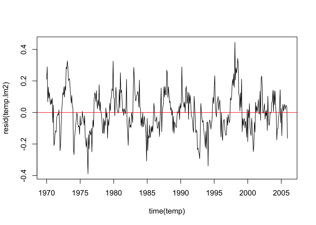

lm2_res <- temp_lm_all |>
  select(lm2) |>
  residuals()
lm2_res |>
  autoplot(.vars = .resid) + 
    geom_hline(yintercept = 0, color = "red")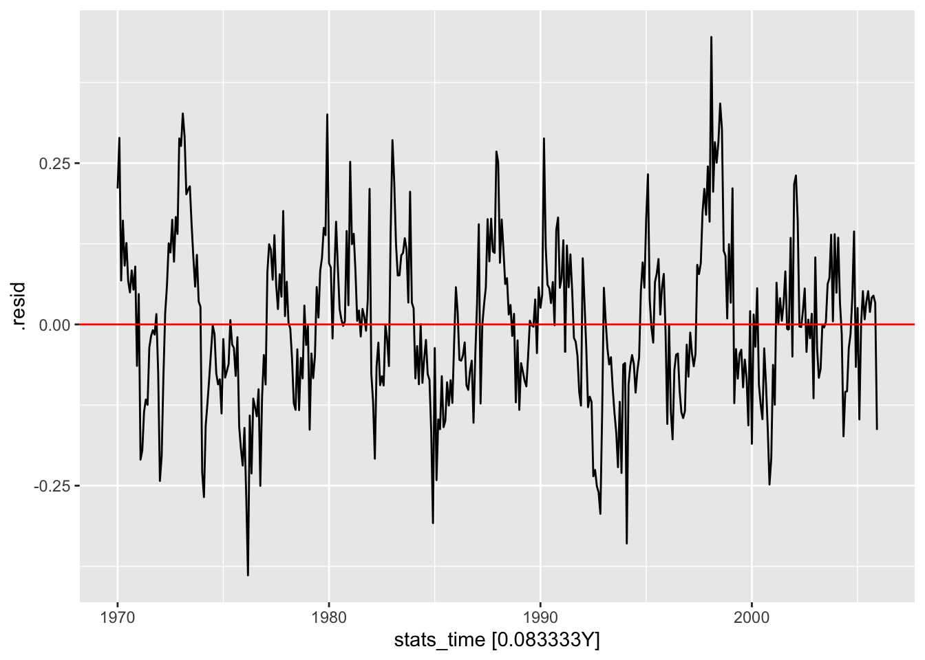

acf(resid(temp.lm2))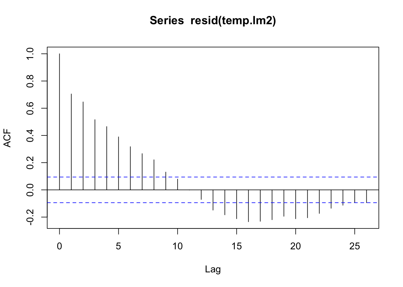

lm2_res |>
  feasts::ACF(var = .resid) |>
  autoplot()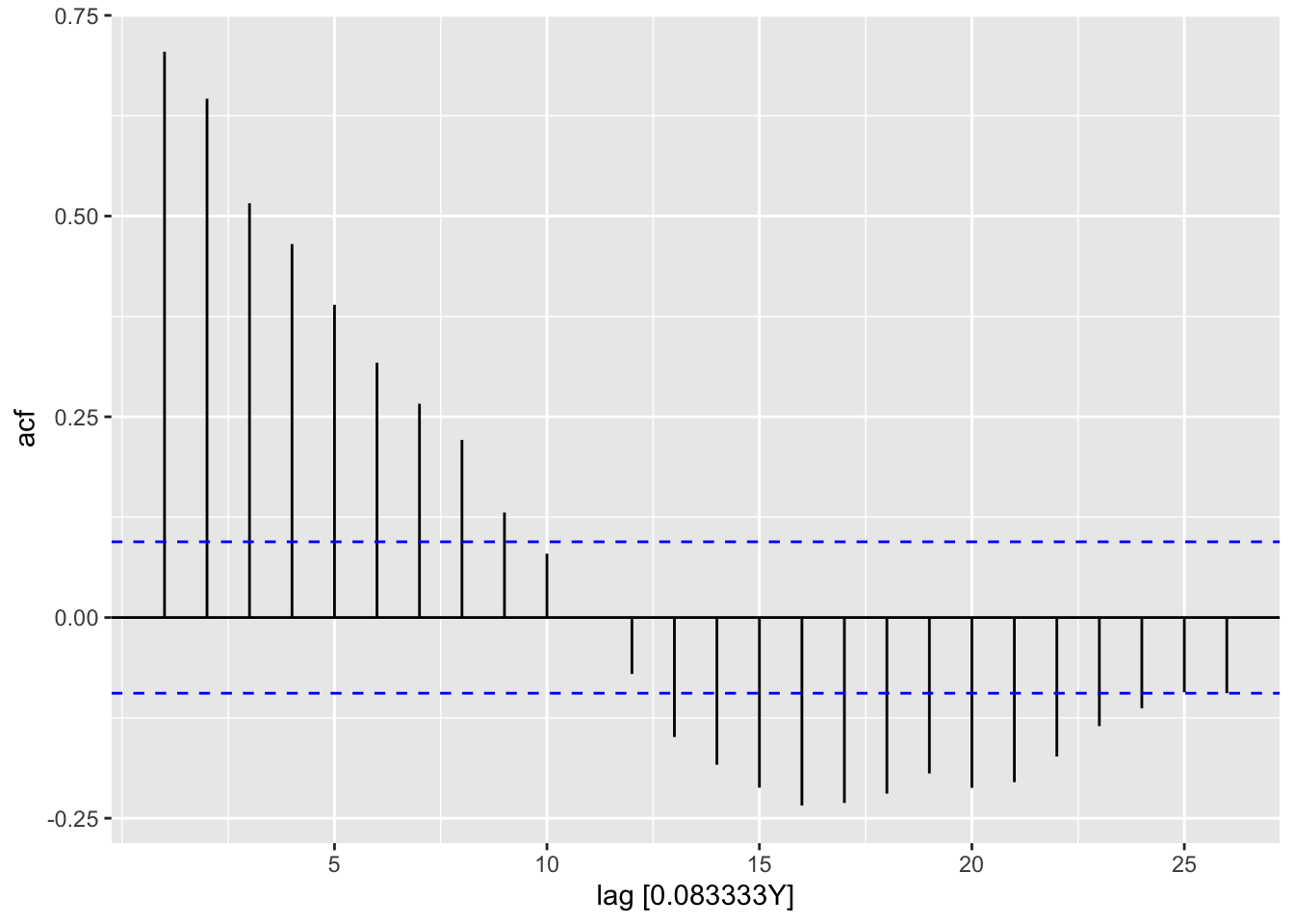

pacf(resid(temp.lm2))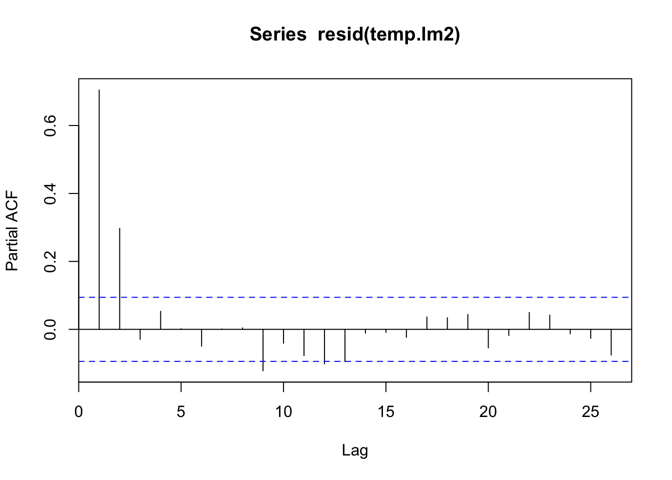

lm2_res |>
  feasts::PACF(var = .resid) |>
  autoplot()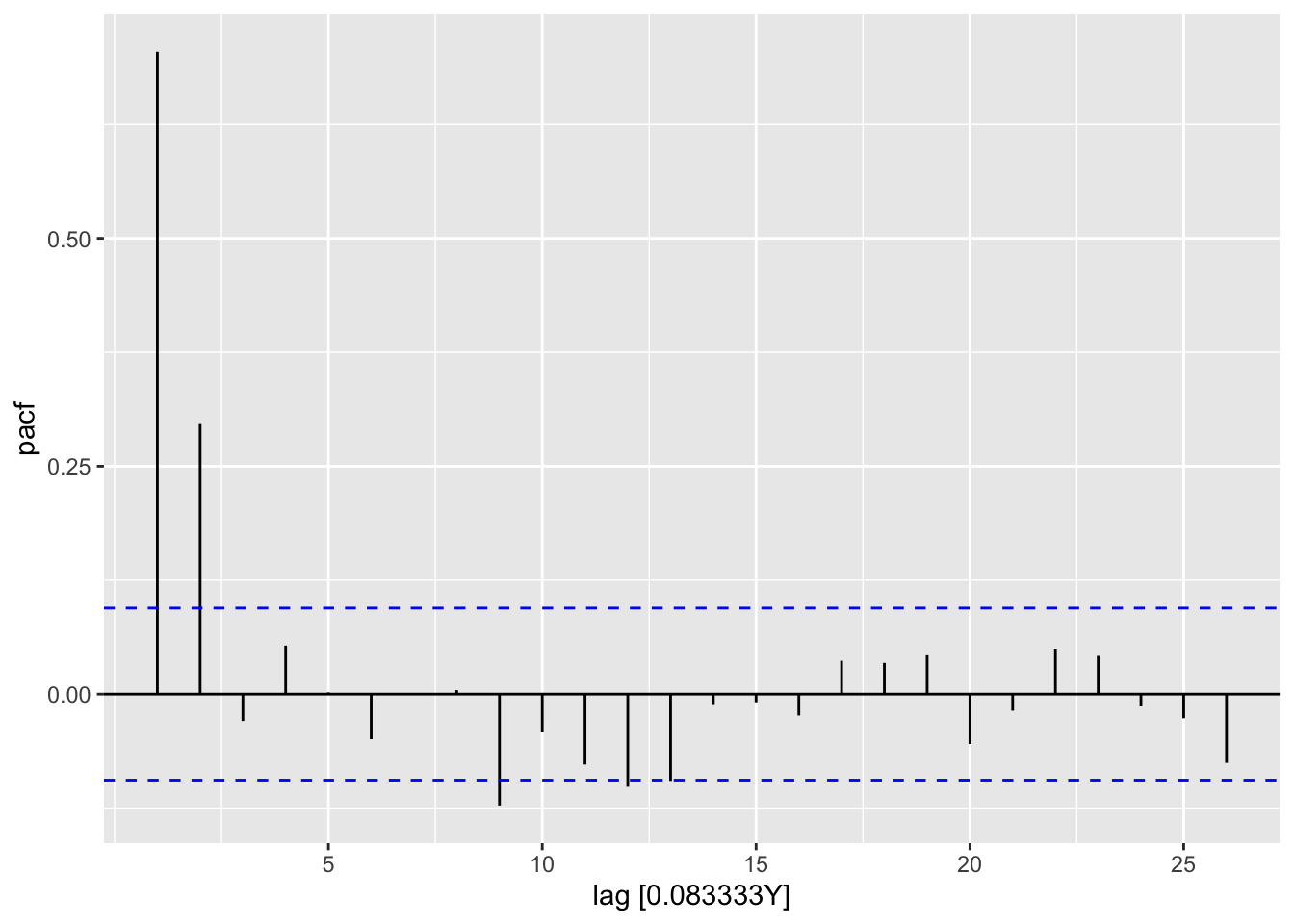

res.ar <- ar(resid(temp.lm2), method = "mle")
res.ar$ar

[1] 0.4938189 0.3071598

res_ar <- lm2_res |>
  select(-.model) |>
  model(resid = AR(.resid ~ order(1:2)))
tidy(res_ar)

# A tibble: 2 × 6
  .model term  estimate std.error statistic  p.value
  <chr>  <chr>    <dbl>     <dbl>     <dbl>    <dbl>
1 resid  ar1      0.486    0.0460     10.6  2.64e-23
2 resid  ar2      0.305    0.0459      6.64 9.30e-11

sd(res.ar$res[-(1:2)])

[1] 0.08373324

sd(pull(residuals(res_ar), .resid), na.rm = TRUE)

[1] 0.08372416

acf(res.ar$res[-(1:2)])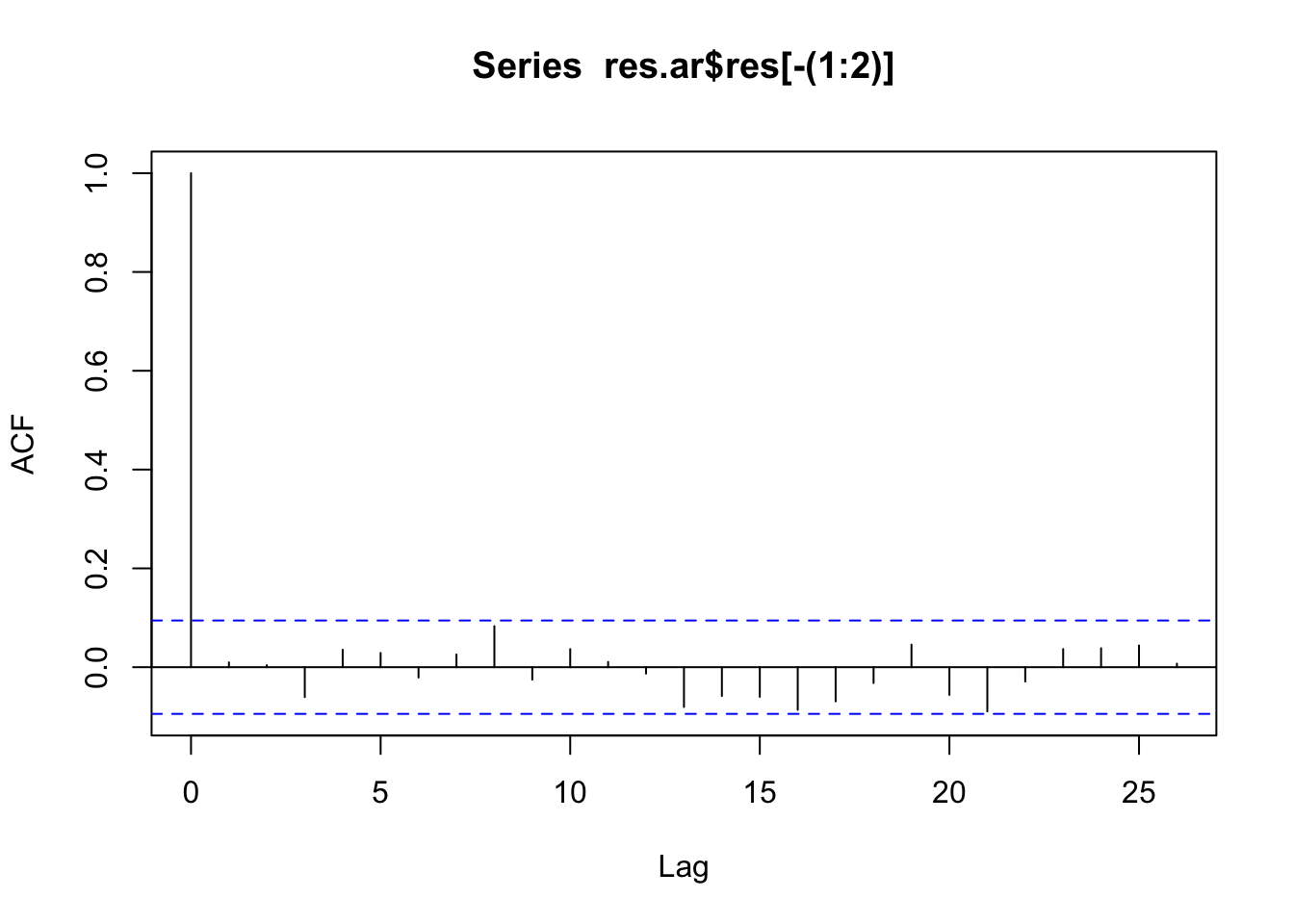

residuals(res_ar) |>
  feasts::ACF(var = .resid) |>
  autoplot()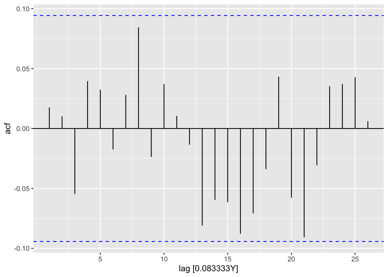

Show the Book code in full

SIN <- COS <- matrix(nr = length(temp), nc = 6)
for (i in 1:6) {
     COS[, i] <- cos(2 * pi * i * time(temp))
     SIN[, i] <- sin(2 * pi * i * time(temp))
 }
TIME <- (time(temp) - mean(time(temp))) / sd(time(temp))
mean(time(temp))
sd(time(temp))
temp.lm1 <- lm(temp ~ TIME + I(TIME^2) +
    COS[,1] + SIN[,1] + COS[,2] + SIN[,2] +
    COS[,3] + SIN[,3] + COS[,4] + SIN[,4] +
    COS[,5] + SIN[,5] + COS[,6] + SIN[,6])
temp.lm2 <- lm(temp ~ TIME + SIN[, 1] + SIN[, 2])
coef(temp.lm1)/sqrt(diag(vcov(temp.lm1)))
coef(temp.lm2)
AIC(temp.lm)
AIC(temp.lm1)
AIC(temp.lm2)
plot(time(temp), resid(temp.lm2), type = "l")
abline(0, 0, col = "red")
acf(resid(temp.lm2))
pacf(resid(temp.lm2))
res.ar <- ar(resid(temp.lm2), method = "mle")
res.ar$ar
sd(res.ar$res[-(1:2)])
acf(res.ar$res[-(1:2)])

Show the Tidyverts code in full

temp_tidy <- temp_tidy |>
  mutate(
    TIME = (stats_time - mean(stats_time)) / sd(stats_time),
    cos1 = cos(2 * pi * 1 * stats_time),
    cos2 = cos(2 * pi * 2 * stats_time),
    cos3 = cos(2 * pi * 3 * stats_time),
    cos4 = cos(2 * pi * 4 * stats_time),
    cos5 = cos(2 * pi * 5 * stats_time),
    cos6 = cos(2 * pi * 6 * stats_time),
    sin1 = sin(2 * pi * 1 * stats_time),
    sin2 = sin(2 * pi * 2 * stats_time),
    sin3 = sin(2 * pi * 3 * stats_time),
    sin4 = sin(2 * pi * 4 * stats_time),
    sin5 = sin(2 * pi * 5 * stats_time),
    sin6 = sin(2 * pi * 6 * stats_time)) |>
  as_tsibble(index = stats_time)
mean(pull(temp_tidy,stats_time))
sd(pull(temp_tidy, stats_time))

temp_lm_all <- temp_tidy |>
  model(
    lm = TSLM(x ~ 0 + stats_time + month),
    lm1 = TSLM(x ~ TIME + I(TIME^2) +
      cos1 + cos2 + cos3 + cos4 + cos5 + cos6 +
      sin1 + sin2 + sin3 + sin4 + sin5 + sin6),
    lm2 = TSLM(x ~ TIME + sin1 + sin2))
temp_lm_all |> select(lm1) |> tidy() |>
  mutate(calc =  estimate / std.error) |>
  select(term, calc)
glance(temp_lm_all) |> select(.model, AIC, AICc, BIC)

lm2_res <- temp_lm_all |>
  select(lm2) |>
  residuals()
lm2_res |>
  autoplot(.vars = .resid) + 
    geom_hline(yintercept = 0, color = "red")
lm2_res |>
  feasts::ACF(var = .resid) |>
  autoplot()
lm2_res |>
  feasts::PACF(var = .resid) |>
  autoplot()
res_ar <- lm2_res |>
  select(-.model) |>
  model(resid = AR(.resid ~ order(1:2)))
tidy(res_ar)
sd(pull(residuals(res_ar), .resid), na.rm = TRUE)
residuals(res_ar) |>
  feasts::ACF(var = .resid) |>
  autoplot()

5.7.2 “Example using the air passenger series” Modern Look

NOTE:

The two full linear models (AP.lm1 and select(ap_lm, lm1)) have slightly different estimates. However, the reduced models match exactly (AP.lm2 and select(ap_lm, lm2)).
The Autogressive fit to the gls models is different. One fits with a mean, and one fits without a mean. Additionally, one is using OLS, and the other is using MLE.

Book code

data(AirPassengers)
AP <- AirPassengers
SIN <- COS <- matrix(nr = length(AP), nc = 6)
for (i in 1:6) {
      SIN[, i] <- sin(2 * pi * i * time(AP))
      COS[, i] <- cos(2 * pi * i * time(AP))
  }

TIME <- (time(AP) - mean(time(AP)))/sd(time(AP))

plot(AP)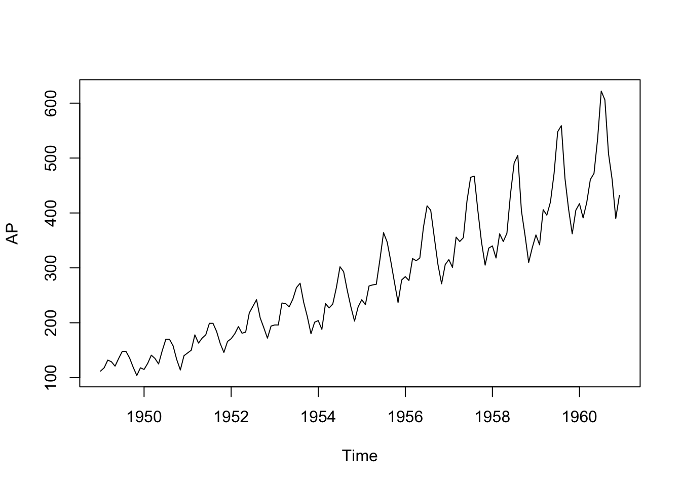

Tidyverts code

data(AirPassengers)
ap <- as_tsibble(AirPassengers)  |>
  mutate(
    Year = year(index),
    Month = month(index),
    stats_time = Year + (Month - 1)/12,
    TIME = (stats_time - mean(stats_time)) / sd(stats_time),
    cos1 = cos(2 * pi * 1 * stats_time),
    cos2 = cos(2 * pi * 2 * stats_time),
    cos3 = cos(2 * pi * 3 * stats_time),
    cos4 = cos(2 * pi * 4 * stats_time),
    cos5 = cos(2 * pi * 5 * stats_time),
    cos6 = cos(2 * pi * 6 * stats_time),
    sin1 = sin(2 * pi * 1 * stats_time),
    sin2 = sin(2 * pi * 2 * stats_time),
    sin3 = sin(2 * pi * 3 * stats_time),
    sin4 = sin(2 * pi * 4 * stats_time),
    sin5 = sin(2 * pi * 5 * stats_time),
    sin6 = sin(2 * pi * 6 * stats_time)) |>
  as_tsibble(index = stats_time)
autoplot(ap)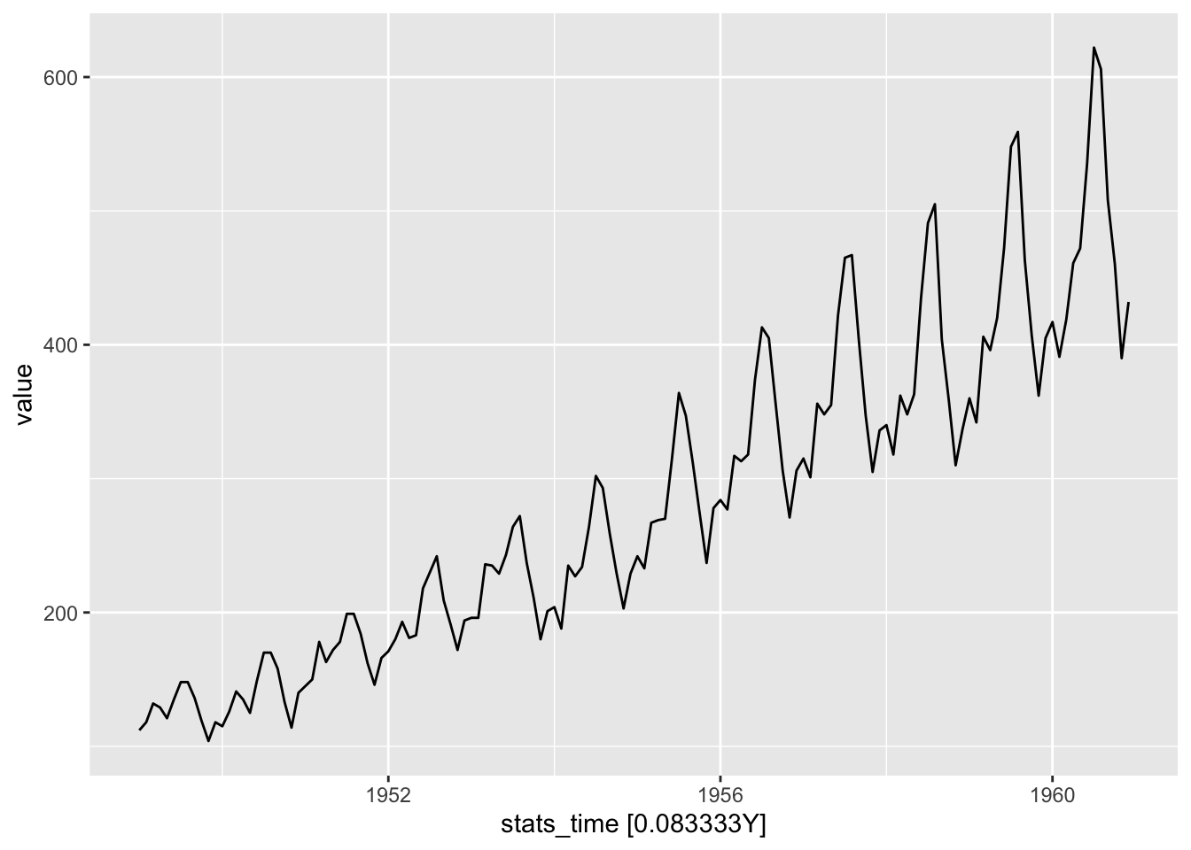

plot(log(AP))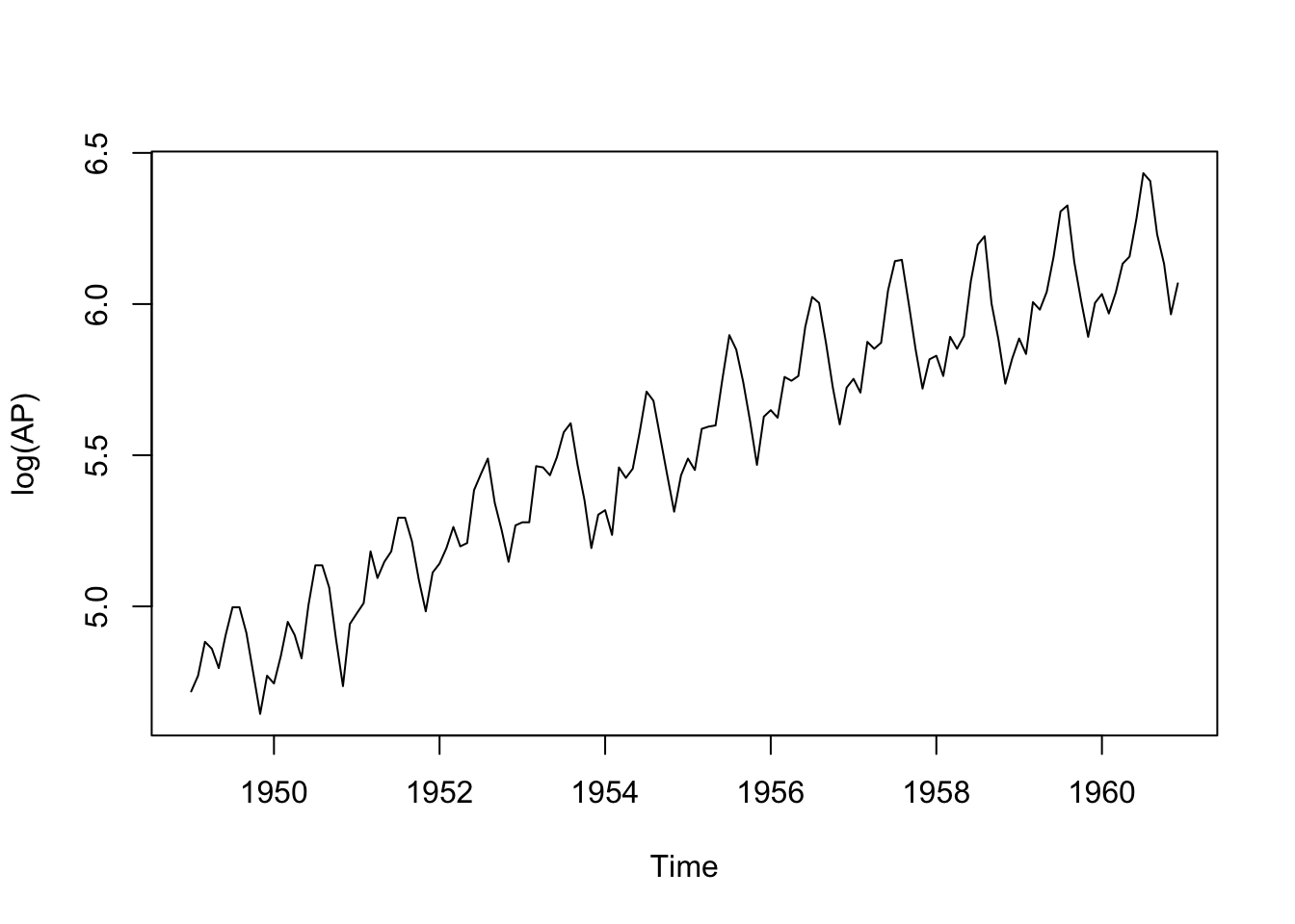

autoplot(ap, .vars = log(value))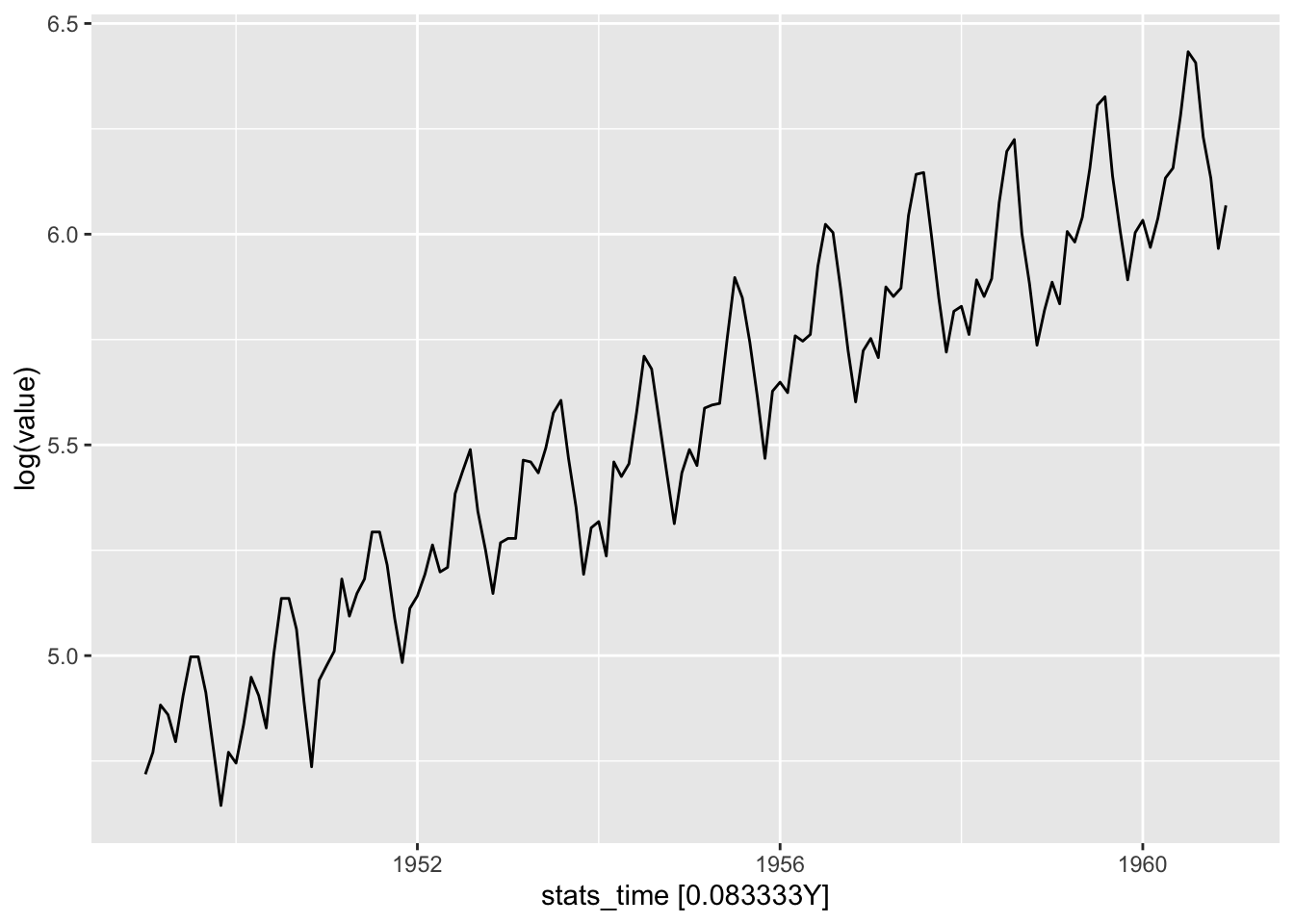

c(mean(time(AP)), sd(time(AP)))

[1] 1954.958333    3.476109

c(mean(pull(ap, stats_time)), 
  sd(pull(ap, stats_time)))

[1] 1954.958333    3.476109

AP.lm1 <- lm(log(AP) ~ TIME + I(TIME^2) + I(TIME^3) +
  I(TIME^4) + SIN[,1] + COS[,1] + SIN[,2] + COS[,2] +
  SIN[,3] + COS[,3] + SIN[,4] + COS[,4] +
  SIN[,5] + COS[,5] + SIN[,6] + COS[,6])
AP.lm2 <- lm(log(AP) ~ TIME + I(TIME^2) +
  SIN[,1] + COS[,1] + SIN[,2] + COS[,2] +
  SIN[,3] + SIN[,4] + COS[,4] + SIN[,5])

list(lm1 = coef(AP.lm1)/sqrt(diag(vcov(AP.lm1))),
  lm2 = coef(AP.lm2)/sqrt(diag(vcov(AP.lm2))))

$lm1
 (Intercept)         TIME    I(TIME^2)    I(TIME^3)    I(TIME^4)     SIN[, 1] 
741.88611010  42.33701405  -4.15995145  -0.74932492   1.86850936   4.86959429 
    COS[, 1]     SIN[, 2]     COS[, 2]     SIN[, 3]     COS[, 3]     SIN[, 4] 
-25.43917945  10.39544938   9.83043452  -4.84196512  -1.51378621  -5.66320251 
    COS[, 4]     SIN[, 5]     COS[, 5]     SIN[, 6]     COS[, 6] 
  1.91354935  -3.76145265   1.01896758   0.07897041  -0.47003062 

$lm2
(Intercept)        TIME   I(TIME^2)    SIN[, 1]    COS[, 1]    SIN[, 2] 
 922.625445  103.520628   -8.235569    4.916041  -25.813114   10.355319 
   COS[, 2]    SIN[, 3]    SIN[, 4]    COS[, 4]    SIN[, 5] 
   9.961335   -4.789997   -5.612235    1.949391   -3.730666

ap_lm <- ap |>
  model(
    lm1 = TSLM(log(value) ~ TIME +
      I(TIME^2) + I(TIME^3) + I(TIME^4) +
      sin1 + cos1 + sin2 + cos2 + sin3 + cos3 +
      sin4 + cos4 + sin5 + cos5 + sin6 + cos6),
    lm2 = TSLM(log(value) ~  TIME + I(TIME^2) + sin1 + cos1 +
    sin2 + cos2 + sin3 + sin4 + cos4 + sin5))

tidy(ap_lm) |>
  mutate(calc = estimate / std.error) |>
  select(.model, term, estimate, std.error, calc) |>
  print(n = 30)

# A tibble: 28 × 5
   .model term        estimate std.error    calc
   <chr>  <chr>          <dbl>     <dbl>   <dbl>
 1 lm1    (Intercept)  5.59e+0   7.50e-3 745.   
 2 lm1    TIME         4.27e-1   1.01e-2  42.4  
 3 lm1    I(TIME^2)   -6.55e-2   1.58e-2  -4.14 
 4 lm1    I(TIME^3)   -3.87e-3   5.19e-3  -0.745
 5 lm1    I(TIME^4)    1.10e-2   5.95e-3   1.85 
 6 lm1    sin1         2.78e-2   5.70e-3   4.87 
 7 lm1    cos1        -1.48e-1   5.67e-3 -26.1  
 8 lm1    sin2         5.92e-2   6.57e-3   9.01 
 9 lm1    cos2         5.66e-2   5.66e-3  10.0  
10 lm1    sin3        -2.74e-2   5.66e-3  -4.84 
11 lm1    cos3        -8.81e-3   5.67e-3  -1.55 
12 lm1    sin4        -3.21e-2   5.66e-3  -5.67 
13 lm1    cos4         1.10e-2   5.66e-3   1.94 
14 lm1    sin5        -2.13e-2   5.67e-3  -3.76 
15 lm1    cos5         5.81e-3   5.66e-3   1.03 
16 lm1    sin6        -1.02e+8   9.91e+8  -0.103
17 lm1    cos6        -3.26e-3   4.76e-3  -0.684
18 lm2    (Intercept)  5.58e+0   6.05e-3 923.   
19 lm2    TIME         4.20e-1   4.06e-3 104.   
20 lm2    I(TIME^2)   -3.74e-2   4.54e-3  -8.24 
21 lm2    sin1         2.81e-2   5.71e-3   4.92 
22 lm2    cos1        -1.47e-1   5.70e-3 -25.8  
23 lm2    sin2         5.91e-2   5.70e-3  10.4  
24 lm2    cos2         5.68e-2   5.70e-3   9.96 
25 lm2    sin3        -2.73e-2   5.70e-3  -4.79 
26 lm2    sin4        -3.20e-2   5.70e-3  -5.61 
27 lm2    cos4         1.11e-2   5.70e-3   1.95 
28 lm2    sin5        -2.13e-2   5.70e-3  -3.73

c(AIC(AP.lm1), AIC(AP.lm2))

[1] -447.9290 -451.0749

glance(ap_lm) |> select(.model, AIC, AICc, BIC)

# A tibble: 2 × 4
  .model   AIC  AICc   BIC
  <chr>  <dbl> <dbl> <dbl>
1 lm1    -857. -851. -803.
2 lm2    -860. -857. -824.

acf(resid(AP.lm2))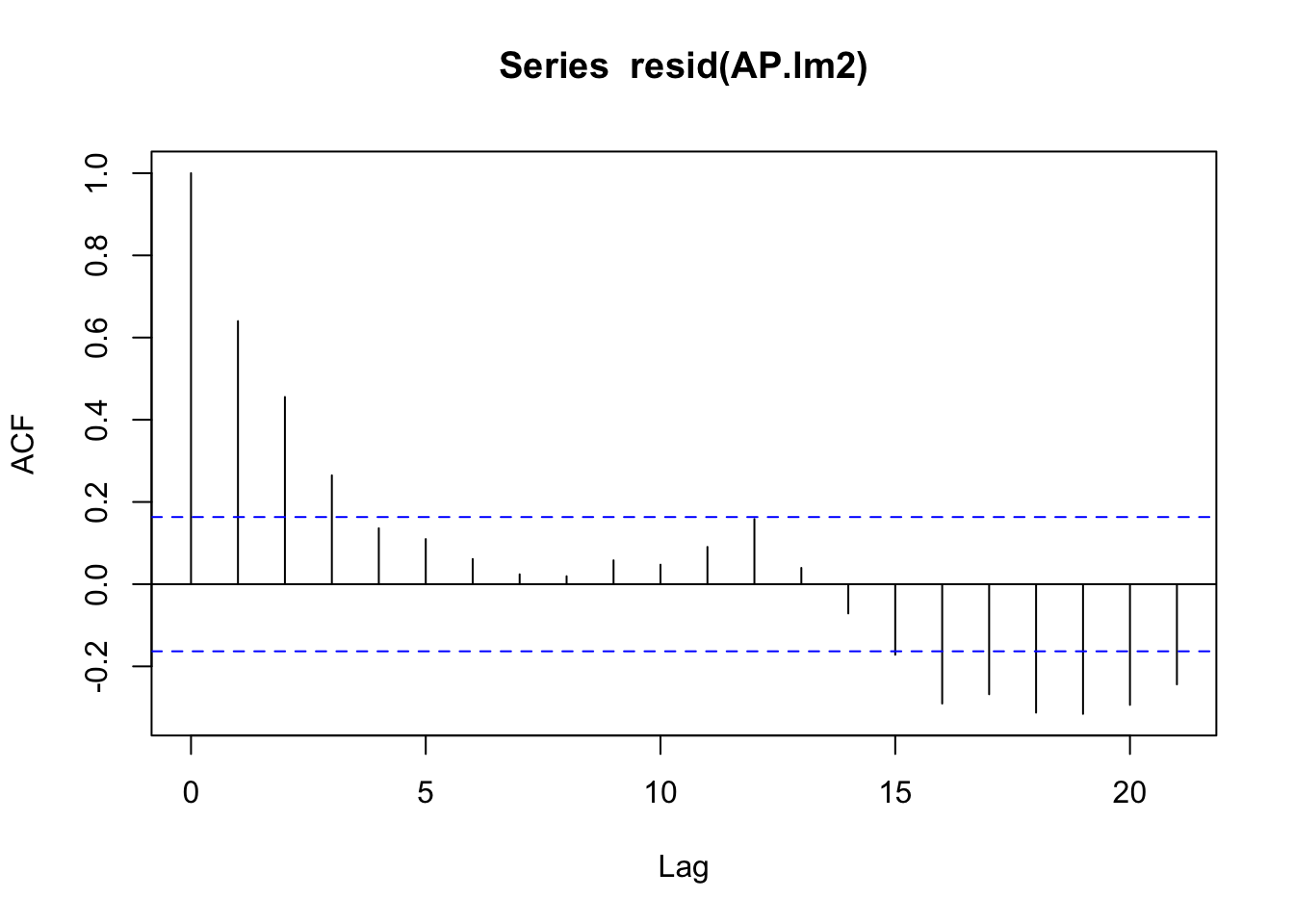

ap_lm |>
  select(lm2) |>
  residuals() |>
  feasts::ACF() |>
  autoplot()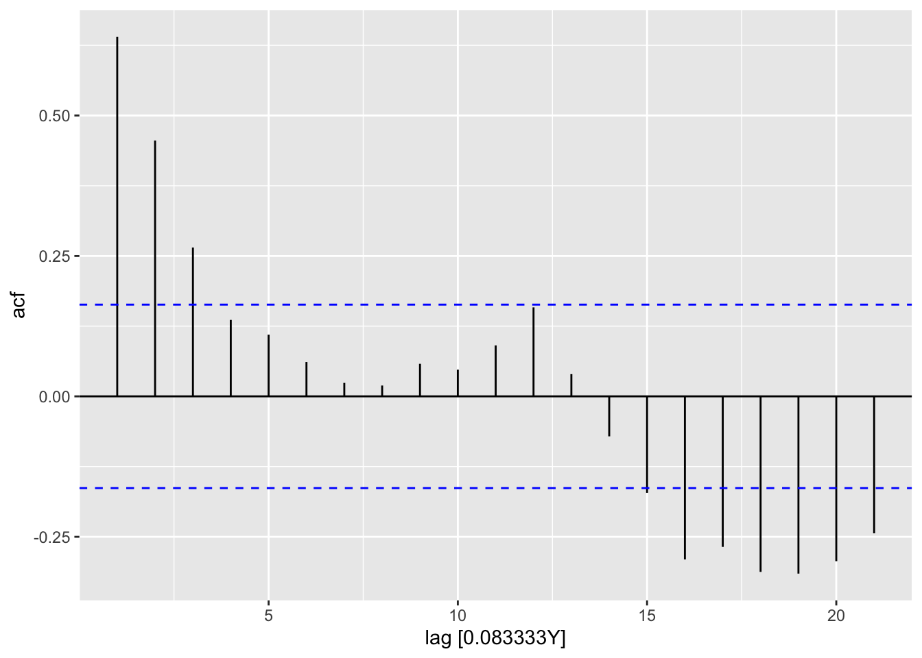

AP.gls <- gls(log(AP) ~ TIME + I(TIME^2) + SIN[,1] + COS[,1] +
     SIN[,2] + COS[,2] + SIN[,3] + SIN[,4] + COS[,4] + SIN[,5],
     cor = corAR1(0.6))
coef(AP.gls)/sqrt(diag(vcov(AP.gls)))

(Intercept)        TIME   I(TIME^2)    SIN[, 1]    COS[, 1]    SIN[, 2] 
 398.841575   45.850520   -3.651287    3.299713  -18.177844   11.768934 
   COS[, 2]    SIN[, 3]    SIN[, 4]    COS[, 4]    SIN[, 5] 
  11.432678   -7.630660  -10.749938    3.571395   -7.920777

ap_gls <- linear_reg() |>
  set_engine("gls", correlation = nlme::corAR1(0.6)) |>
  fit(log(value) ~  TIME + I(TIME^2) + sin1 + cos1 +
    sin2 + cos2 + sin3 + sin4 + cos4 + sin5, data = ap)

broom.mixed::tidy(ap_gls) |>
  mutate(calc = estimate / std.error) |>
  select(term, estimate, std.error, calc)

# A tibble: 11 × 4
   term        estimate std.error   calc
   <chr>          <dbl>     <dbl>  <dbl>
 1 (Intercept)   5.58     0.0140  399.  
 2 TIME          0.418    0.00913  45.9 
 3 I(TIME^2)    -0.0364   0.00996  -3.65
 4 sin1          0.0270   0.00819   3.30
 5 cos1         -0.147    0.00810 -18.2 
 6 sin2          0.0584   0.00496  11.8 
 7 cos2          0.0565   0.00494  11.4 
 8 sin3         -0.0277   0.00363  -7.63
 9 sin4         -0.0322   0.00300 -10.7 
10 cos4          0.0107   0.00301   3.57
11 sin5         -0.0214   0.00270  -7.92

AP.ar <- ar(resid(AP.lm2), order = 1, method = "mle")
AP.ar$ar

[1] 0.6410685

ap_ar <- augment(ap_gls, ap) |>
  as_tsibble(index = stats_time) |>
  model(resid = AR(.resid ~ order(1)))

tidy(ap_ar)

# A tibble: 2 × 6
  .model term     estimate std.error statistic  p.value
  <chr>  <chr>       <dbl>     <dbl>     <dbl>    <dbl>
1 resid  constant   13.5      6.97        1.94 5.50e- 2
2 resid  ar1         0.959    0.0234     41.1  1.14e-80

acf(AP.ar$res[-1])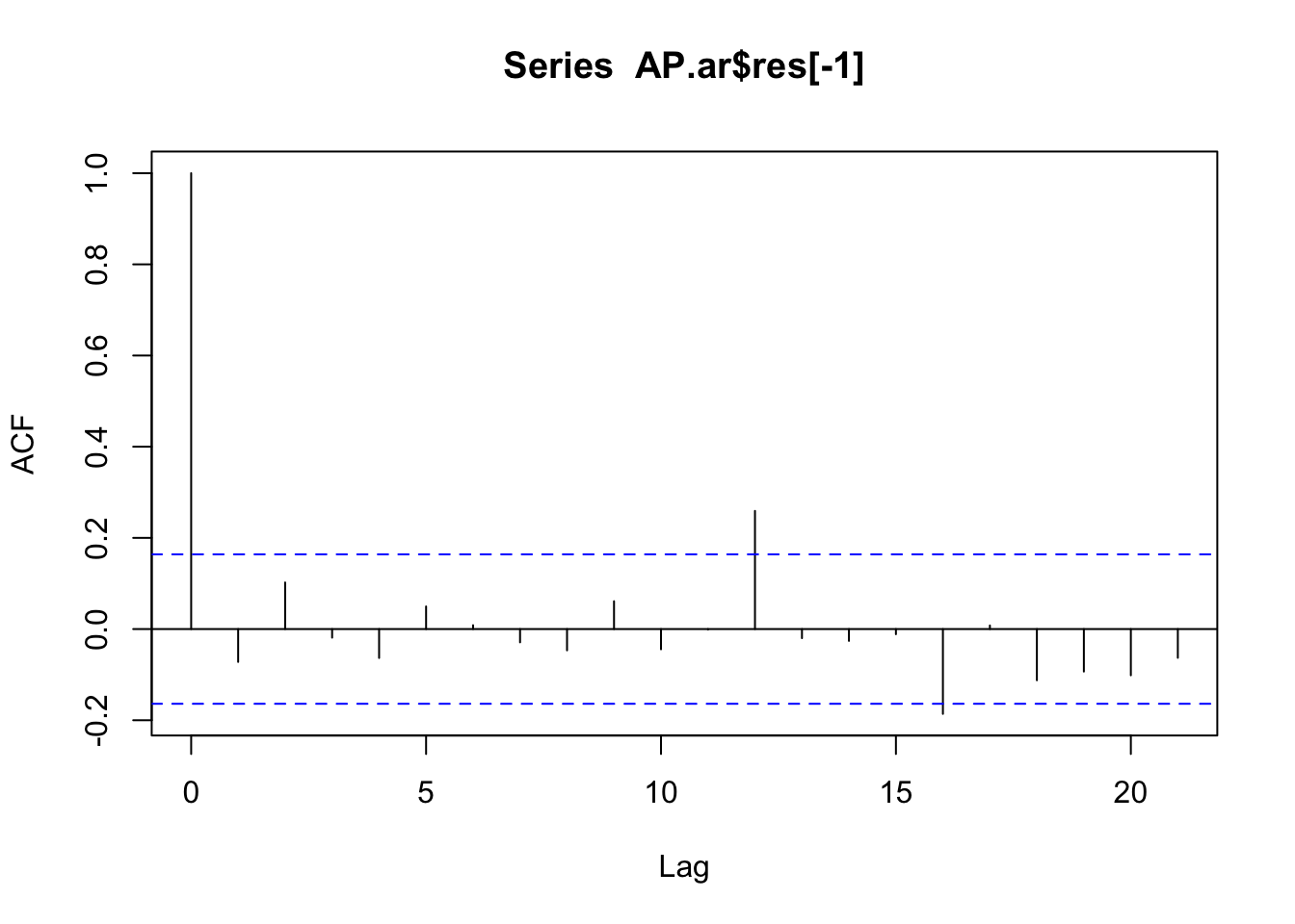

residuals(ap_ar) |>
  feasts::ACF(.var = .resid) |>
  autoplot()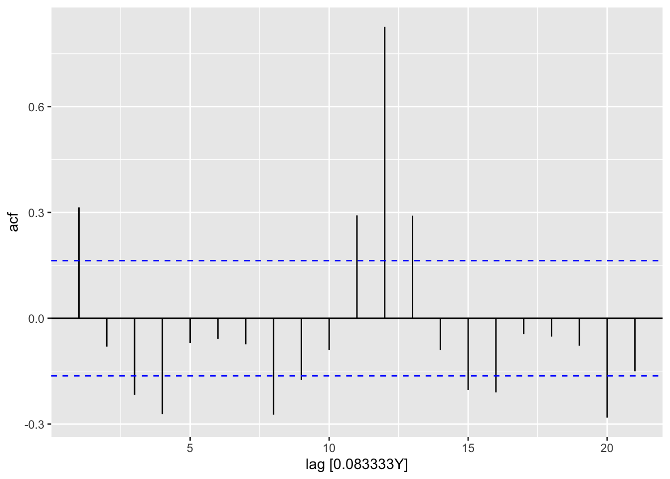

Show the Book code in full

data(AirPassengers)
AP <- AirPassengers
SIN <- COS <- matrix(nr = length(AP), nc = 6)
for (i in 1:6) {
      SIN[, i] <- sin(2 * pi * i * time(AP))
      COS[, i] <- cos(2 * pi * i * time(AP))
  }
TIME <- (time(AP) - mean(time(AP)))/sd(time(AP))

plot(AP)
plot(log(AP))

mean(time(AP))
sd(time(AP))

AP.lm1 <- lm(log(AP) ~ TIME + I(TIME^2) + I(TIME^3) + I(TIME^4) +
         SIN[,1] + COS[,1] + SIN[,2] + COS[,2] + SIN[,3] + COS[,3] +
         SIN[,4] + COS[,4] + SIN[,5] + COS[,5] + SIN[,6] + COS[,6])
AP.lm2 <- lm(log(AP) ~ TIME + I(TIME^2) + SIN[,1] + COS[,1] +
    SIN[,2] + COS[,2] + SIN[,3] + SIN[,4] + COS[,4] + SIN[,5])

list(lm1 = coef(AP.lm1)/sqrt(diag(vcov(AP.lm1))),
  lm2 = coef(AP.lm2)/sqrt(diag(vcov(AP.lm2))))

c(AIC(AP.lm1), AIC(AP.lm2))

acf(resid(AP.lm2))

AP.gls <- gls(log(AP) ~ TIME + I(TIME^2) + SIN[,1] + COS[,1] +
     SIN[,2] + COS[,2] + SIN[,3] + SIN[,4] + COS[,4] + SIN[,5],
     cor = corAR1(0.6))
coef(AP.gls)/sqrt(diag(vcov(AP.gls)))
AP.ar <- ar(resid(AP.lm2), order = 1, method = "mle")
AP.ar$ar
acf(AP.ar$res[-1])

Show the Tidyverts code in full

data(AirPassengers)
ap <- as_tsibble(AirPassengers)  |>
  mutate(
    Year = year(index),
    Month = month(index),
    stats_time = Year + (Month - 1)/12,
    TIME = (stats_time - mean(stats_time)) / sd(stats_time),
    cos1 = cos(2 * pi * 1 * stats_time),
    cos2 = cos(2 * pi * 2 * stats_time),
    cos3 = cos(2 * pi * 3 * stats_time),
    cos4 = cos(2 * pi * 4 * stats_time),
    cos5 = cos(2 * pi * 5 * stats_time),
    cos6 = cos(2 * pi * 6 * stats_time),
    sin1 = sin(2 * pi * 1 * stats_time),
    sin2 = sin(2 * pi * 2 * stats_time),
    sin3 = sin(2 * pi * 3 * stats_time),
    sin4 = sin(2 * pi * 4 * stats_time),
    sin5 = sin(2 * pi * 5 * stats_time),
    sin6 = sin(2 * pi * 6 * stats_time)) |>
  as_tsibble(index = stats_time)
autoplot(ap)
autoplot(ap, .vars = log(value))

mean(pull(ap, stats_time))
sd(pull(ap, stats_time))

ap_lm <- ap |>
  model(
    lm1 = TSLM(log(value) ~ TIME +
      I(TIME^2) + I(TIME^3) + I(TIME^4) +
      sin1 + cos1 + sin2 + cos2 + sin3 + cos3 +
      sin4 + cos4 + sin5 + cos5 + sin6 + cos6),
    lm2 = TSLM(log(value) ~  TIME + I(TIME^2) + sin1 + cos1 +
    sin2 + cos2 + sin3 + sin4 + cos4 + sin5))

tidy(ap_lm) |>
  mutate(calc = estimate / std.error) |>
  print(n = 30)

glance(ap_lm) |> select(.model, AIC, AICc, BIC)

ap_lm |>
  select(lm2) |>
  residuals() |>
  feasts::ACF() |>
  autoplot()


ap_gls <- linear_reg() |>
  set_engine("gls", correlation = nlme::corAR1(0.6)) |>
  fit(log(value) ~  TIME + I(TIME^2) + sin1 + cos1 +
    sin2 + cos2 + sin3 + sin4 + cos4 + sin5, data = ap)

broom.mixed::tidy(ap_gls) |>
  mutate(calc = estimate / std.error)

ap_ar <- augment(ap_gls, ap) |>
  as_tsibble(index = stats_time) |>
  model(resid = AR(.resid ~ order(1)))

tidy(ap_ar)

residuals(ap_ar) |>
  feasts::ACF(.var = .resid) |>
  autoplot()

5.8.2 “Example of a simulated and fitted non-linear series” Modern Look

Book code

set.seed(1)
w <- rnorm(100, sd = 10)
z <- rep(0, 100)
for (t in 2:100) z[t] <- 0.7 * z[t - 1] + w[t]
Time <- 1:100
f <- function(x) exp(1 + 0.05 * x)
x <- f(Time) + z
plot(x, type = "l")
abline(0, 0)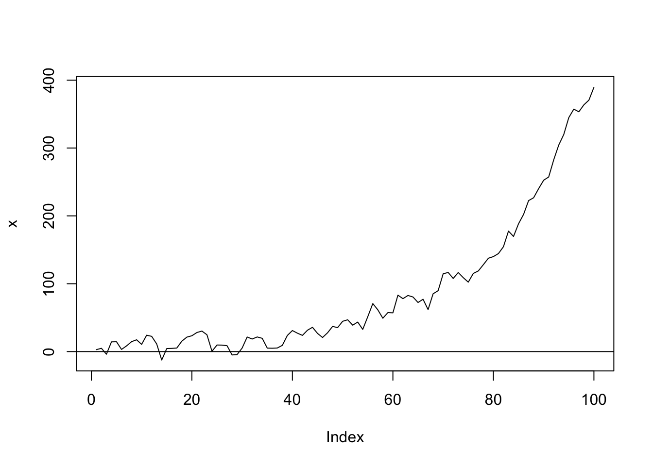

Tidyverts code

set.seed(1)
dat <- tibble(w = rnorm(100, sd = 10)) |>
    mutate(
        Time = 1:n(),
         z = purrr::accumulate2(
            lag(w), w, 
            \(acc, nxt, w) 0.7 * acc + w,
            .init = 0)[-1],
          x = exp(1 + 0.05 * Time) + z) |>
    tsibble::as_tsibble(index = Time)

autoplot(dat, .var = x) +
  geom_hline(yintercept = 0)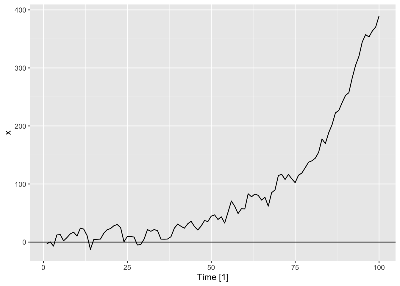

x.nls <- nls(x ~ exp(alp0 + alp1 * Time), start = list(alp0 = 0.1,
      alp1 = 0.5))
summary(x.nls)$parameters

       Estimate   Std. Error  t value     Pr(>|t|)
alp0 1.17640121 0.0742954459 15.83410 9.204061e-29
alp1 0.04828424 0.0008188462 58.96619 2.347546e-78

equation <- x ~ exp(alp0 + alp1 * Time)

dat_nls <- nls(equation, data = dat,
  start = list(alp0 = 0.1, alp1 = 0.5))
summary(dat_nls)$parameters

       Estimate   Std. Error  t value     Pr(>|t|)
alp0 1.17299000 0.0743864847 15.76886 1.232132e-28
alp1 0.04832158 0.0008197862 58.94413 2.432829e-78

Show the Book code in full

set.seed(1)
w <- rnorm(100, sd = 10)
z <- rep(0, 100)
for (t in 2:100) z[t] <- 0.7 * z[t - 1] + w[t]
Time <- 1:100
f <- function(x) exp(1 + 0.05 * x)
x <- f(Time) + z
plot(x, type = "l")
abline(0, 0)
x.nls <- nls(x ~ exp(alp0 + alp1 * Time), start = list(alp0 = 0.1,
      alp1 = 0.5))
summary(x.nls)$parameters

Show the Tidyverts code in full

set.seed(1)
dat <- tibble(w = rnorm(100, sd = 10)) |>
    mutate(
        Time = 1:n(),
         z = purrr::accumulate2(
            lag(w), w, 
            \(acc, nxt, w) 0.7 * acc + w,
            .init = 0)[-1],
          x = exp(1 + 0.05 * Time) + z) |>
    tsibble::as_tsibble(index = Time)

autoplot(dat, .var = x) +
  geom_hline(yintercept = 0)

equation <- x ~ exp(alp0 + alp1 * Time)

dat_nls <- nls(equation, data = dat,
  start = list(alp0 = 0.1, alp1 = 0.5))
summary(dat_nls)$parameters

5.9.2 “Prediction in R” Modern Look

Book code

new.t <- time(ts(start = 1961, end = c(1970, 12), fr = 12))
TIME <- (new.t - mean(time(AP)))/sd(time(AP))
SIN <- COS <- matrix(nr = length(new.t), nc = 6)
for (i in 1:6) {
      COS[, i] <- cos(2 * pi * i * new.t)
      SIN[, i] <- sin(2 * pi * i * new.t)
  }
SIN <- SIN[, -6]
new.dat <- data.frame(TIME = as.vector(TIME), SIN = SIN,
      COS = COS)
AP.pred.ts <- exp(ts(predict(AP.lm2, new.dat), st = 1961,
      fr = 12))
ts.plot(log(AP), log(AP.pred.ts), lty = 1:2)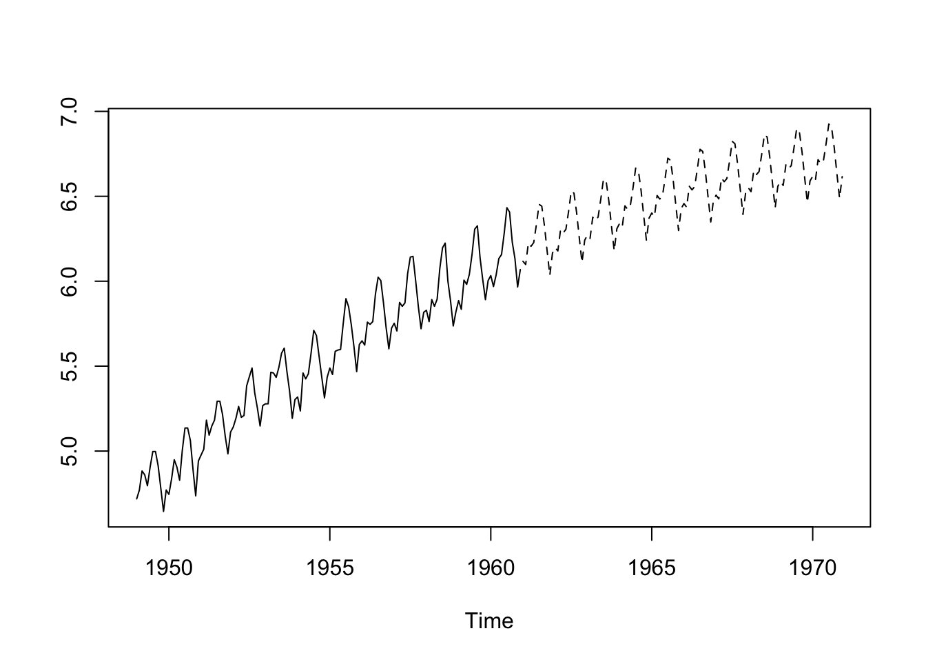

Tidyverts code

new_dat <- tibble(new_t = seq(1961, 1970.99, 1/12)) |>
  mutate(
    TIME = (new_t - mean(pull(ap, stats_time))) / sd(pull(ap, stats_time)),
    cos1 = cos(2 * pi * 1 * new_t),
    cos2 = cos(2 * pi * 2 * new_t),
    cos3 = cos(2 * pi * 3 * new_t),
    cos4 = cos(2 * pi * 4 * new_t),
    cos5 = cos(2 * pi * 5 * new_t),
    cos6 = cos(2 * pi * 6 * new_t),
    sin1 = sin(2 * pi * 1 * new_t),
    sin2 = sin(2 * pi * 2 * new_t),
    sin3 = sin(2 * pi * 3 * new_t),
    sin4 = sin(2 * pi * 4 * new_t),
    sin5 = sin(2 * pi * 5 * new_t)) |>
  rename(stats_time = new_t) |>
  as_tsibble(index = stats_time)

ap_lm |> 
  select(lm2) |>
  forecast(new_data = new_dat) |>
  autoplot(ap, level = 95) +
    scale_y_continuous(trans = "log", labels = trans_format("log"))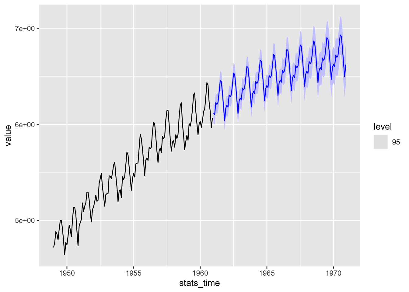

ts.plot(AP, AP.pred.ts, lty = 1:2)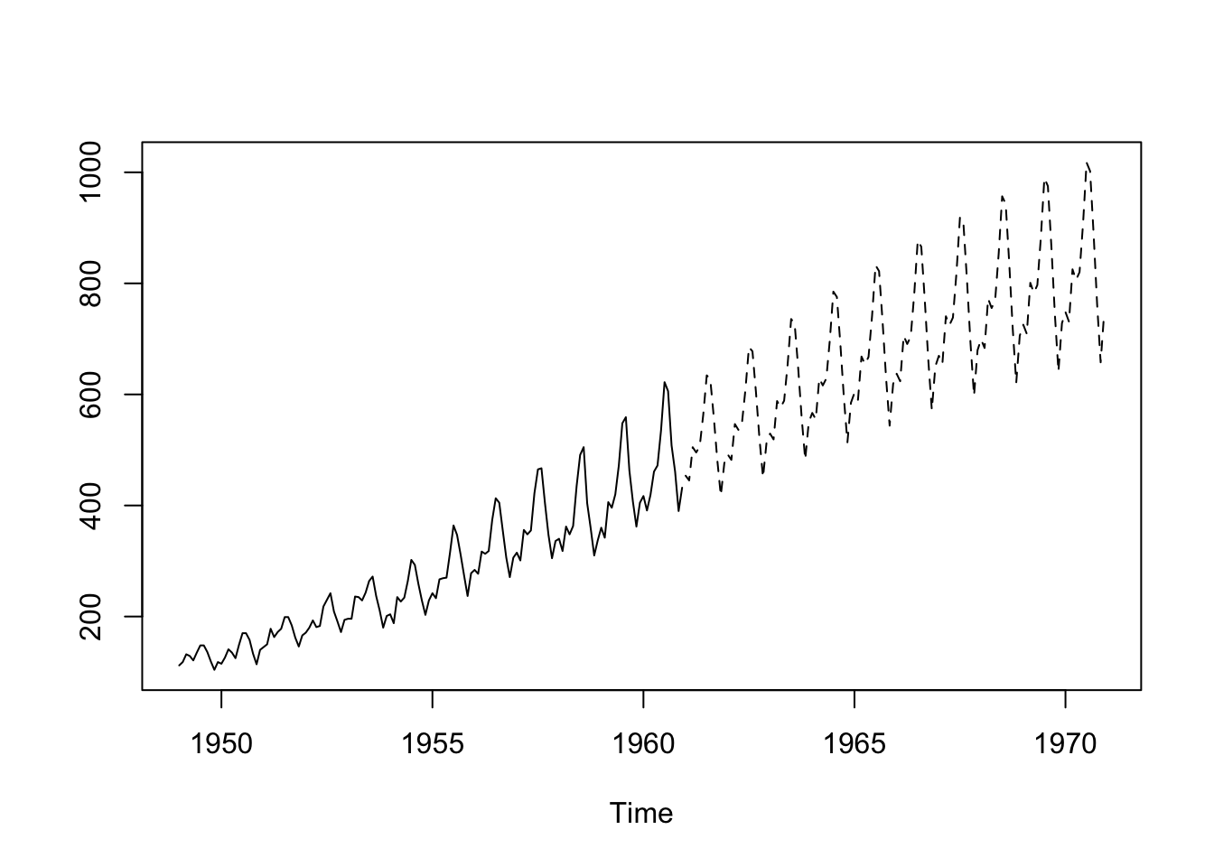

ap_lm |> 
  select(lm2) |>
  forecast(new_data = new_dat) |>
  autoplot(ap, level = 95)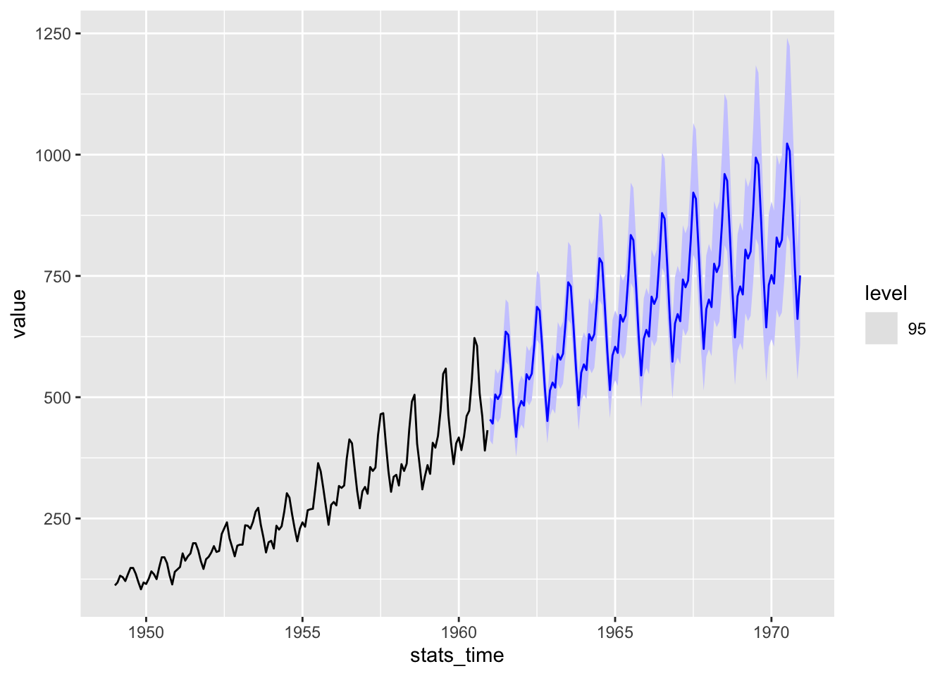

Show the Book code in full

new.t <- time(ts(start = 1961, end = c(1970, 12), fr = 12))
TIME <- (new.t - mean(time(AP)))/sd(time(AP))
SIN <- COS <- matrix(nr = length(new.t), nc = 6)
for (i in 1:6) {
      COS[, i] <- cos(2 * pi * i * new.t)
      SIN[, i] <- sin(2 * pi * i * new.t)
  }
SIN <- SIN[, -6]
new.dat <- data.frame(TIME = as.vector(TIME), SIN = SIN,
      COS = COS)
AP.pred.ts <- exp(ts(predict(AP.lm2, new.dat), st = 1961,
      fr = 12))
ts.plot(log(AP), log(AP.pred.ts), lty = 1:2)
ts.plot(AP, AP.pred.ts, lty = 1:2)

Show the Tidyverts code in full

new_dat <- tibble(new_t = seq(1961, 1970.99, 1/12)) |>
  mutate(
    TIME = (new_t - mean(pull(ap, stats_time))) / sd(pull(ap, stats_time)),
    cos1 = cos(2 * pi * 1 * new_t),
    cos2 = cos(2 * pi * 2 * new_t),
    cos3 = cos(2 * pi * 3 * new_t),
    cos4 = cos(2 * pi * 4 * new_t),
    cos5 = cos(2 * pi * 5 * new_t),
    cos6 = cos(2 * pi * 6 * new_t),
    sin1 = sin(2 * pi * 1 * new_t),
    sin2 = sin(2 * pi * 2 * new_t),
    sin3 = sin(2 * pi * 3 * new_t),
    sin4 = sin(2 * pi * 4 * new_t),
    sin5 = sin(2 * pi * 5 * new_t)) |>
  rename(stats_time = new_t) |>
  as_tsibble(index = stats_time)

ap_lm |> 
  select(lm2) |>
  forecast(new_data = new_dat) |>
  autoplot(ap, level = 95) +
    scale_y_continuous(trans = "log", labels = trans_format("log"))

ap_lm |> 
  select(lm2) |>
  forecast(new_data = new_dat) |>
  autoplot(ap, level = 95)

5.10.1 “Log-normal residual errors” Modern Look

Book code

set.seed(1)
sigma <- 1
w <- rnorm(1e+06, sd = sigma)
c(mean(w), mean(exp(w)), exp(sigma^2/2))

[1] 4.690776e-05 1.648610e+00 1.648721e+00

Tidyverts code

set.seed(1)
sigma <- 1
w <- rnorm(1e+06, sd = sigma)
c(mean(w), mean(exp(w)), exp(sigma^2/2))

[1] 4.690776e-05 1.648610e+00 1.648721e+00

Show the Book code in full

set.seed(1)
sigma <- 1
w <- rnorm(1e+06, sd = sigma)
c(mean(w), mean(exp(w)), exp(sigma^2/2))

Show the Tidyverts code in full

set.seed(1)
sigma <- 1
w <- rnorm(1e+06, sd = sigma)
c(mean(w), mean(exp(w)), exp(sigma^2/2))

5.10.3 Example using the air passenger data

Book code

summary(AP.lm2)$r.sq

[1] 0.9888318

Tidyverts code

model_values <- ap_lm |>
  select(lm2) |>
  glance()
model_values |>
  select(r_squared)

# A tibble: 1 × 1
  r_squared
      <dbl>
1     0.989

sigma <- summary(AP.lm2)$sigma
lognorm.correction.factor <- exp((1/2) * sigma^2)
empirical.correction.factor <- mean(exp(resid(AP.lm2)))
c(lognorm.correction.factor, empirical.correction.factor)

[1] 1.001171 1.001080

old <- options(pillar.sigfig = 7)
model_check <- model_values |>
  mutate(
    sigma = sqrt(sigma2),
    lognorm_cf = exp((1/2) * sigma2),
    empirical_cf = ap_lm |>
      select(lm2) |>
      residuals() |>
      pull(.resid) |>
      exp() |>
      mean()) |>
  select(.model, r_squared, sigma2, sigma, lognorm_cf, empirical_cf)
model_check

# A tibble: 1 × 6
  .model r_squared      sigma2      sigma lognorm_cf empirical_cf
  <chr>      <dbl>       <dbl>      <dbl>      <dbl>        <dbl>
1 lm2    0.9888318 0.002340141 0.04837501   1.001171     1.001080

AP.pred.ts <- AP.pred.ts * empirical.correction.factor

options(old)
ap_pred <- ap_lm |> 
  select(lm2) |>
  forecast(new_data = new_dat) |>
  mutate(.mean_correction = .mean * model_check$empirical_cf) |>
  select(stats_time, value, .mean, .mean_correction)

Show the Book code in full

summary(AP.lm2)$r.sq
sigma <- summary(AP.lm2)$sigma
lognorm.correction.factor <- exp((1/2) * sigma^2)
empirical.correction.factor <- mean(exp(resid(AP.lm2)))
c(lognorm.correction.factor, empirical.correction.factor)
AP.pred.ts <- AP.pred.ts * empirical.correction.factor

Show the Tidyverts code in full

model_values <- ap_lm |>
  select(lm2) |>
  glance()
model_values |>
  select(r_squared)

old <- options(pillar.sigfig = 7)
model_check <- model_values |>
  mutate(
    sigma = sqrt(sigma2),
    lognorm_cf = exp((1/2) * sigma2),
    empirical_cf = ap_lm |>
      select(lm2) |>
      residuals() |>
      pull(.resid) |>
      exp() |>
      mean()) |>
  select(.model, r_squared, sigma2, sigma, lognorm_cf, empirical_cf)
model_check
options(old)

ap_pred <- ap_lm |> 
  select(lm2) |>
  forecast(new_data = new_dat) |>
  mutate(.mean_correction = .mean * model_check$empirical_cf) |>
  select(stats_time, value, .mean, .mean_correction)

5.11 Summary of Modern `R` commands used in examples

fable::TSLM(): Fit a linear model with time series components
parsnip::linear_reg(): Linear regression
parsnip::set_engine(): Declare a computational engine and specific arguments
nlme::corAR1: AR(1) Correlation Structure
broom.mixed::tidy(): Turn an object into a tidy tibble
broom::glance(): Glance at a(n) lm object
ggplot2::geom_hline(): Reference lines: horizontal, vertical, and diagonal
ggplot2::scale_y_continuous(): Position scales for continuous data (x & y)
scales::trans_format(): Format labels after transformation

5.2.3 “Simulation in R” Modern Look

5.3.1 “Model fitted to simulated data” Modern Look

5.3.1 “Model fitted to the temperature series (1970-2005)” Modern Look

5.4.1 “GLS fit to simulated series” Modern Look

5.4.2 “Confidence interval for the trend in the temperature series” Modern Look

5.5.3 “Example: Seasonal model for the temperature series” Modern Look

5.6 “Harmonic seasonal models” Modern Look

5.6.1 “Simulation” Modern Look

5.6.2 “Fit to simulated series” Modern Look

5.6.3 “Harmonic model fitted to temperature series (1970–2005)” Modern Look

5.7.2 “Example using the air passenger series” Modern Look

5.8.2 “Example of a simulated and fitted non-linear series” Modern Look

5.9.2 “Prediction in R” Modern Look

5.10.1 “Log-normal residual errors” Modern Look

5.10.3 Example using the air passenger data

5.11 Summary of Modern R commands used in examples

5.2.3 “Simulation in `R`” Modern Look

5.11 Summary of Modern `R` commands used in examples