Lesson 19 Inference for Independence of Categorical Data

Optional Videos for this Lesson

Part 1

Part 2

Part 3

Part 4

Lesson Outcomes

By the end of this lesson, you should be able to do the following.

1. Recognize when a chi-square test for independence is appropriate
2. Create numerical and graphical summaries of the data
3. Perform a hypothesis test for the chi-square test for independence using the following steps:
   1. State the null and alternative hypotheses
   2. Calculate the test-statistic, degrees of freedom and P-value of the test using software
   3. Assess statistical significance in order to state the appropriate conclusion for the hypothesis test
   4. Check the requirements for the hypothesis test
4. State the properties of the chi-square distribution

The \(\chi^2\) (Chi-squared) Test of Independence

People often wonder whether two things influence each other. For example, people seek chiropractic care for different reasons. We may want to know if those reasons are different for Europeans than for Americans or Australians. This question can be expressed as “Do reasons for seeking chiropractic care depend on the location in which one lives?”

This question has only two possible answers: “yes” and “no.” The answer “no” can be written as “Motivations for seeking chiropractic care and one’s location are independent.” (The statistical meaning of “independent” is too technical to give here. However, for now, you can think of it as meaning that the two variables are not associated in any way. For example, neither variable depends on the other.) Writing the answer “no” this way allows us to use it as the null hypothesis of a test. We can write the alternative hypothesis by expressing the answer “yes” as “Motivations for seeking chiropractic care and one’s location are not independent.” (Reasons for wording it this way will be given after you’ve been through the entire hypothesis test.)

To prepare for the hypothesis test, recall that our hypothesis tests always measure how different two or more things are. For example, in the 2-sample \(t\)-test, we compare two population means by seeing how different they are. In a test of one proportion, we measure the difference between a sample proportion and a population proportion. Each of these tests requires some information about at least one parameter. That information is given in the null hypothesis of the test, which we’ve always been able to write with one or more “=” signs, because we’ve always used numeric parameters.

Unfortunately, we have no parameter we can use to measure the independence of the variables “location” and “motivation”. Nevertheless, we have to be able to calculate a \(P\)-value, and the only approach we have so far is to measure differences between things. “Difference” means “subtraction” in Statistics, and if the measurements are categorical, we cannot subtract them. Therefore, as in the other lessons of this unit, we will count occurrences of each value of each variable to get some numbers. (The example that follows will show how this is handled.) The numbers we get will be called “counts” or “observed counts”.

When we have our observed counts in hand, software will calculate the counts we should expect to see, if the null hypothesis is true. We call these the “expected counts.” The software will then subtract the observed counts from the expected counts and combine these differences to create a single number that we can use to get a \(P\)-value. That single number is called the \(\chi^2\) test statistic. (Note that \(\chi\) is a Greek letter, and its name is “ki”, as in “kite”. The symbol \(\chi^2\) should be pronounced “ki squared,” but many people pronounce it “ki-square.”)

In this course, software will calculate the \(\chi^2\) test statistic for you, but you need to understand that the \(\chi^2\) test statistic compares the observed counts to the expected counts—that is, to the counts we should expect to get if the null hypothesis is true. The larger the \(\chi^2\) test statistic is, the smaller the \(P\)-value will be. If the \(\chi^2\) test statistic is large enough that the \(P\)-value is less than \(\alpha\), we will conclude that the observed counts and expected counts are too different for the null hypothesis to be plausible, and will therefore reject \(H_0\). Otherwise, we will fail to reject \(H_0\), as always.

For organizational reasons, counts are traditionally arranged in a table called a “contingency table.” One variable is chosen as the “row variable,” so called because its values are the row headers for the table. The other variable is called the “column variable,” because its values are the column headers. Different \(\chi^2\) distributions are distinguished by the number of degrees of freedom, which are determined by the number of rows and columns in the table:

\[df = (\text{number of rows }-1)(\text{number of columns }-1)\]

Note that the number of degrees of freedom does not depend on the number of subjects in the study.

Reasons for Seeking Chiropractic Care

A study was conducted to determine why patients seek chiropractic care. Patients were classified based on their location and their motivation for seeking treatment. Using descriptions developed by Green and Krueter, patients were asked which of the five reasons led them to seek chiropractic care :

• Wellness: defined as optimizing health among the self-identified healthy
• Preventive health: defined as preventing illness among the self-identified healthy
• At risk: defined as preventing illness among the currently healthy who are at heightened risk to develop a specific condition
• Sick role: defined as getting well among those self-perceived as ill with an emphasis on therapist-directed treatment
• Self care: defined as getting well among those self-perceived as ill favoring the use of self vs. therapist directed strategies

The data from the study are summarized in the following contingency table :

Motivation

Location	Wellness	Preventive Health	At Risk	Sick Role	Self Care	Total
Europe	23	28	59	77	95	282
Australia	71	59	83	68	188	469
United States	90	76	65	82	252	565
Total	184	163	207	227	535	1316

The research question was whether people’s motivation for seeking chiropractic care was independent of their location: Europe, Australia, or the United States. The hypothesis test used to address this question was the chi-squared (\(\chi^2\)) test of independence. (Recall that the Greek letter \(\chi\) is pronounced, “ki” as in “kite.”)

Excel Instructions

• In the Excel sheet Math 221 Statistics Toolbox, go to the tab labeled “Chi Squared”. This tab will allow you to perform tests for independence. Excel allows us to enter data in the same way as the table above, so enter the data in the following manner on the excel sheet:

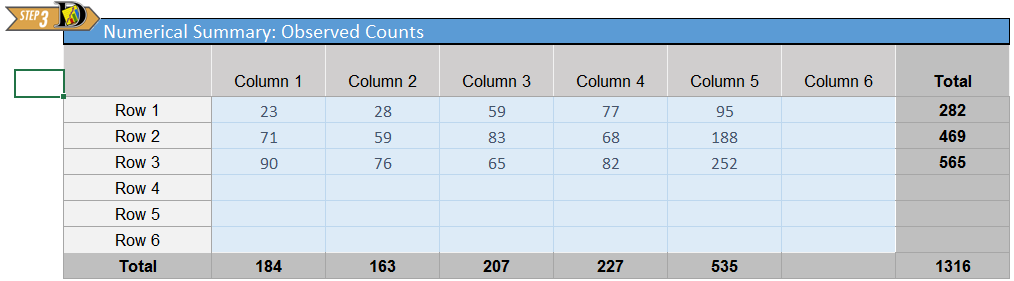
• Note: The boxes without data are left blank.
  

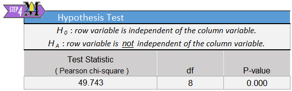
The null and alternative hypotheses for this chi-squared test of independence are: \[ \begin{array}{rl} H_0\colon & \text{The location and the motivation for seeking treatment are independent} \\ H_a\colon & \text{The location and the motivation for seeking treatment are not independent} \\ \end{array} \]

Note: When speaking of the hypotheses in the absence of a context, we can write them in the form \[ \begin{array}{rl} H_0\colon & \text{The row variable and the column variable are independent} \\ H_a\colon & \text{The row variable and the column variable are not independent.} \\ \end{array} \] But when there’s a context, please make sure you write your hypotheses in terms of the context.

If the row and column variable are independent, then no matter which row you consider, the proportion of observations in each column should be roughly the same. For example, if motivation for seeking chiropractic care is independent of location, then the proportion of people who seek chiropractic care for, say, wellness will be approximately the same in each row. That is, it will be approximately the same for Australians, Europeans, and Americans.

Excel Instructions

• The Chi-Square statistic, degrees of freedom, and \(P\)-value of the hypotheiss test are all displayed to the right of the where the data is entered in. The data for this example will look like:

• If we reject the null hypothesis, we state, “There is sufficient evidence to suggest that (restate the alternative hypothesis.)” If we failed to reject the null hypothesis, we would replace the word, “sufficient” with “insufficient.”

Requirements

The following requirements must be met in order to conduct a \(\chi^2\) test of independence:

1. You must use simple random sampling to obtain a sample from a single population.
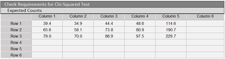
2. Each expected count must be greater than or equal to 5.

A table of expected counts is found starting in cell S4 (scroll to the right of the data entry area and hypothesis test results).

Let’s walk through the chiropractic example now from beginning to end:

Background:

• Context of the study: The population of interest consisted of chiropractic patients in three locations: Australia, Europe, and the United States. The objective was to determine whether reasons for seeking chiropractic care are different in the different locations.
• Research question: Is a patient’s location independent of their motivation for seeking treatment? In other words, do people in Australia, Europe, and the United States seek chiropractic care for the same reasons?
• Data collection procedures: Upon check-in at their visit, patients were provided a brief questionnaire regarding the reason they were seeking care. Responses were categorized and tabulated. (Note that the table contains statistics (frequencies) that describe the patients in the sample.)

Descriptive statistics:

Motivation

Location	Wellness	Preventive Health	At Risk	Sick Role	Self Care	Total
Europe	23	28	59	77	95	282
Australia	71	59	83	68	188	469
United States	90	76	65	82	252	565
Total	184	163	207	227	535	1316

Inferential statistics:

The appropriate hypothesis test is the chi-squared test for independence. The requirement that the expected counts are all at least 5 is met. (Check the picture of the Expected Counts table already shown above.)

Conduct the hypothesis test:

\(~~~~~H_0\colon\) Location and the motivation to visit a chiropractor are independent.

\(~~~~~H_a\colon\) Location and the motivation to visit a chiropractor are not independent.

Let \(\alpha=0.05\).

The test statistic is: \(\chi^2 = 49.743\), with \(df=8\).

The \(P\)-value is rounded to .000 in the output. To see the actual \(P\)-value you would need to use Excel to expand the number of decimal places shown: \(P\textrm{-value} = 4.58 \times 10^{-8} < 0.05 = \alpha\)

Decision: Reject the null hypothesis.

Conclusion: There is sufficient evidence to suggest that the motivation to visit a chiropractor is not independent of the location.

Other considerations

Swapping the Row and Column Variables

There is no general guideline for deciding which variable is the row variable and which variable is the column variable in a \(\chi^2\) test of independence. To see why not, complete the questions that follow.

Answer the following questions:

1. Re-do the \(\chi^2\) test of independence for the chiropractic care data, but use “Motivation” as the row variable. Then compare the degrees of freedom, \(\chi^2\) test statistic, and \(P\)-value of this test, with the degrees of freedom, \(\chi^2\) test statistic, and \(P\)-value for the test conducted above, when “Location” was the row variable.

Show/Hide Solution

• In both tests, \(df = 8\), \(\chi^2 = 49.743\), and the \(P\)-value is \(4.58 \times 10^{-8} < 0.05 = \alpha\). They are the same for both tests.

2. What do you conclude about swapping the row and column variables in a \(\chi^2\) test of independence?

Show/Hide Solution

• Swapping the row and column variables in a \(\chi^2\) test of independence does not change the conclusion of the test.

 

There may be no general guideline for deciding which variable is the row variable, but the graphics produced by your software may depend on this decision. For example, Excel will give you a different clustered bar chart when you use “Location” as the row variable than when you use “Motivation” as the row variable. Sometimes, choosing one of the variables as the row variable makes the clustered bar chart easier to understand. The bar chart is just below the data entry area in Excel.

Why \(H_a\) is Worded As It Is

Recall that in the chiropractic care example, the hypotheses for the \(\chi^2\) test of independence were

\(H_0\colon\) Location and the motivation to visit a chiropractor are independent. \(H_a\colon\) Location and the motivation to visit a chiropractor are not independent.

You may wonder why we don’t write “\(H_a\colon\) The motivation to visit a chiropractor depends on location.” Well, couldn’t we say just as easily that location depends on the motivation to visit a chiropractor? It may seem a little strange when phrased this way. Let’s use the following exercises to look briefly at a somewhat less strange example, then return to this example.

Answer the following questions:

3. Suppose you want to know whether a student’s stress level and the degree to which they feel a need to succeed are independent. What should your hypotheses be?

Show/Hide Solution

• \(H_0\colon\) Stress level and the need to succeed are independent.
• \(H_a\colon\) Stress level and the need to succeed are not independent.

4. For their alternative hypothesis, a student erroneously writes “\(H_a\colon\) Stress level depends on the need to succeed.” If they reject \(H_0\), what will they conclude?

Show/Hide Solution

• They will conclude that a student’s stress level depends on their need to succeed.

5. Another student erroneously writes “\(H_a\colon\) Need to succeed depends on stress levels.” If they reject \(H_0\), what will they conclude?

Show/Hide Solution

• They will conclude that the degree to which a student feels a need to succeed depends on their stress level.

6. Could it be that a student’s need to succeed depends on their stress level? Could it be that their stress level depends on their need to succeed? How can the \(\chi^2\) test of independence distinguish between these two possibilities?

Show/Hide Solution

• Students that feel a more intense need to succeed than others might very well experience higher stress levels. Likewise, a student who feels their stress levels rising might subconsiously feel that success will decrease their stress level, which could result in their feeling an increased need to succeed.

• The \(\chi^2\) test statistic and the \(P\)-value will be the same, whether we write down the correct alternative hypothesis or one of the two erroneous ones mentioned above. The \(\chi^2\) test of independence is not capable of telling whether stress levels depend on the need to succeed or whether the need to succeed depends on the stress level.

• If swapping the row and column variables made a difference in the outcome of the hypothesis test, then the test might be able to tell which variable depends on the other. But swapping the row and column variables does not change the outcome of the test.

• The full truth is worse than this: It may be that one’s need to succeed and one’s stress level depend on each other. It may be that neither depends on the other, but that both depend on something else, in a way that makes it look like they depend on each other. The \(\chi^2\) test of independence is incapable of distinguishing among the many possible kinds of dependence.

 

According to the exercises you just did, we are not justified in writing an alternative hypothesis that specifies which variable depends on which. Could we write “\(H_a\colon\) Stress level and need to succeed are dependent”? After all, “independent” and “dependent” are opposites, aren’t they? This may seem reasonable, but we have to be careful of the technical terms. Statisticians have gone to some trouble to carefully define “independent.” They have not defined “dependent.” (As suggested by the exercises you just did, dependence is complicated, perhaps too complicated to be able to be defined conveniently.) They use the phrase “not independent” as the opposite of “independent.” So will we, writing “\(H_a\colon\) Stress level and need to succeed are not independent.”

Likewise, in the chiropractic care example, we can’t say in the alternative hypothesis that location depends on motivation, nor that motivation depends on location, nor that each depends on the other, nor that both depend on something else, nor that location and motivation are dependent. Instead, we write “\(H_a\colon\) The location and the motivation for seeking treatment are not independent,” as statisticians do.

No Confidence Intervals

We do not calculate confidence intervals when working with contingency tables. Think about it: With three rows and five columns in the table for the chiropractic care example, there are 15 proportions, which means there would be 105 pairs of proportions to compare. How could we possibly interpret a collection of 105 confidence intervals? Also, if our confidence level is 95%, we would expect that about 5 of our confidence intervals would not contain the true difference between proportions, but we wouldn’t know which ones. Rather than take the risks this would cause, the Statistics culture has agreed not to calculate confidence intervals for contingency tables.

Summary

Remember…

• The \(\chi^2\) hypothesis test is a test of independence between two variables. These variables are either associated or they are not. Therefore, the null and alternative hypotheses are the same for every test: \[ \begin{array}{1cl} H_0: & \text{The (first variable) and the (second variable) are independent.} \\ H_a: & \text{The (first variable) and the (second variable) are not independent.} \end{array} \]

• The degrees of freedom (\(df\)) for a \(\chi^2\) test of independence are calculated using the formula \(df=(\text{number of rows}-1)(\text{number of columns}-1)\)

• In our hypothesis testing for \(\chi^2\) we never conclude that two variables are dependent. Instead, we say that two variables are not independent.
  

Navigation

Previous Reading	This Reading	Next Reading
Lesson 18: Inference for Two Proportions	Lesson 19: Inference for Independence of Categorical Data	Lesson 20: Review for Exam 3

---

Copyright © 2020 Brigham Young University-Idaho. All rights reserved.