Lesson 11 Inference for One Mean (Sigma Unknown)

Optional Videos for this Lesson

Part 1

Part 2

Part 3

Part 4

Lesson Outcomes

By the end of this lesson, you should be able to do the following:

1. Recognize when a one mean (sigma unknown) inferential procedure is appropriate
2. Create numerical and graphical summaries of the data
3. Perform a hypothesis test for one mean (sigma unknown) using the following steps:
   1. State the null and alternative hypotheses
   2. Calculate the test-statistic, degrees of freedom and P-value using software
   3. Assess statistical significance in order to state the appropriate conclusion for the hypothesis test
   4. Check the requirements for the hypothesis test
4. Create a confidence interval for one mean (sigma unknown) using the following steps:
   1. Calculate a confidence interval for a given level of confidence using software
   2. Interpret the confidence interval
   3. Check the requirements of the confidence interval
5. State the properties of the Student’s t-distribution

What If We Don’t Know \(\sigma\)?

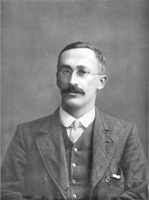
In practice, we almost never know the population standard deviation, \(\sigma\). So, it is generally not appropriate to use the formula \[ z = \frac{ \bar x - \mu }{ \sigma / \sqrt{n} } \] In 1908, William Sealy Gosset published a solution to this problem. He found a way to appropriately compute the confidence interval for the mean when \(\sigma\) is not known. The basic idea is to use the sample standard deviation, \(s\), in the place of the true population standard deviation, \(\sigma\). If \(\sigma\) is not known, we cannot base the calculations on the standard normal distribution, and we cannot use the formula above to conduct hypothesis tests.

In a remarkable piece of work, Gosset found the appropriate distribution to use when \(\sigma\) is unknown. At the time of this discovery, Gosset worked for the Guinness brewery. To avoid problems with industrial espionage, Guinness prohibited employees from publishing any research results. Knowing his work provided a significant contribution to Statistics, Gosset convinced his employer to allow him to publish under a fictitious name. He chose the pseudonym “Student”. Gosset’s test statistic was denoted by the letter \(t\), this distribution has come to be known as Student’s t-distribution.

\[ t = \frac{ \bar x - \mu }{ s / \sqrt{n} } \]

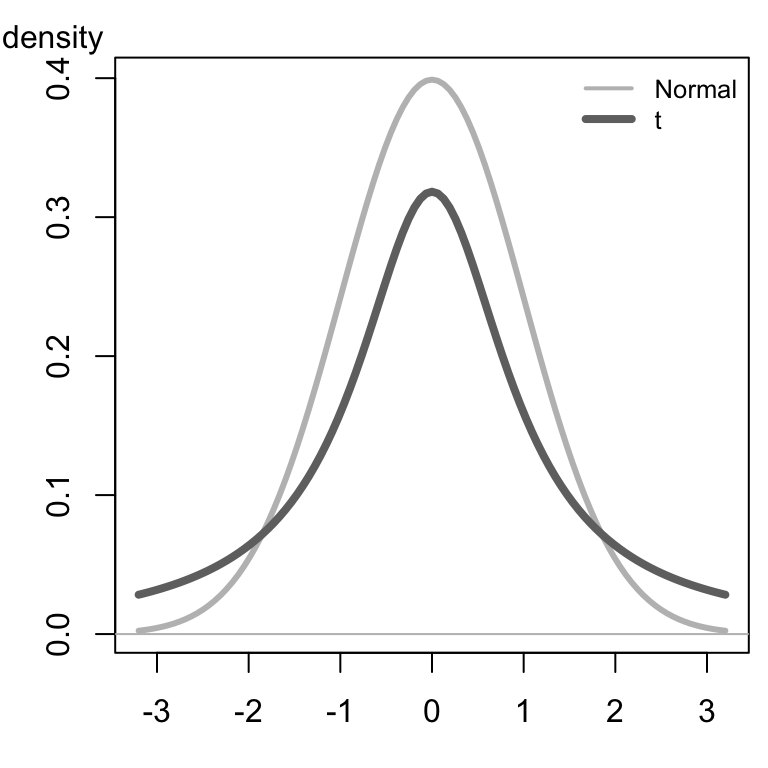
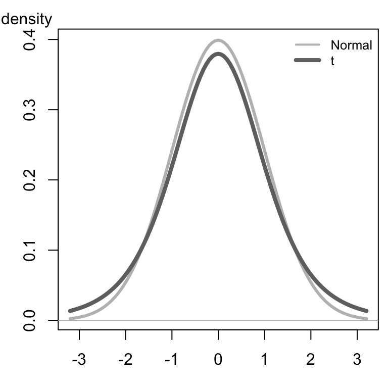
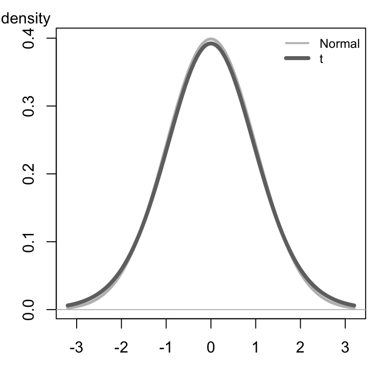
The \(t\)-distribution is bell-shaped and symmetrical. The \(t\)-distribution has a mean of 0, but it has more area in the tails than the standard normal distribution. The exact shape of the \(t\)-distribution depends on a parameter called the degrees of freedom (abbreviated \(df\)). The degrees of freedom is related to the sample size. As the sample size goes up, the degrees of freedom increase accordingly. For the procedures discussed in this lesson, the degrees of freedom is one less than the sample size: \(df = n-1\).

Click here to explore how the shape of the \(t\)-distribution changes with the degrees of freedom. Notice that as the degrees of freedom increases, the shape of the \(t\)-distribution (dark curve) gets closer to the standard normal distribution (lighter curve). The lighter gray curve is identical (always normal) in the three images below, while the darker curve changes shape as the degrees of freedom increase.

\(t\)-distribution with \(df = 1\)	\(t\)-distribution with \(df = 5\)	\(t\)-distribution with \(df = 15\)

Hypothesis Tests

Body Temperatures Revisited

We will apply the \(t\)-distribution to the body temperature data we explored previously.

This hypothesis test is conducted in a manner similar to a test for a single mean where \(\sigma\) is known, except that instead of using the population standard deviation, \(\sigma\), in the calculations, we estimate this value using the sample standard deviation, \(s\). This leads to a \(t\)-distribution, rather than a normal distribution for the test statistic. We will not need to compute the value of this test statistic by hand. It will be done using Software.

Summarize the relevant background information

We want to conduct a hypothesis test to determine if the mean body temperature is different from 98.6° Fahrenheit. Previously, we assumed that we knew the value of \(\sigma\). Actually, this value is not known.

State the null and alternative hypotheses and the level of significance

\[ \begin{array}{rl} H_0: \mu = 98.6\\ H_a: \mu \ne 98.6\\ \end{array} \]

\[ \alpha = 0.05 \]

Describe the data collection procedures

We will use the body temperature data, BodyTemp.xlsx, collected by Dr. Mackowiak and his colleagues to conduct the test.

Give the relevant summary statistics

\[ \begin{array}{l} \bar x = 98.23\\ s = 0.738\\ n = 148 \end{array} \]

Make an appropriate graph (e.g. a histogram) to illustrate the data

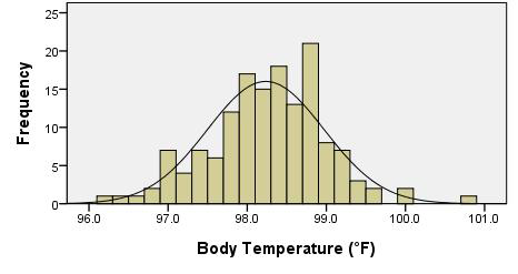
Verify the requirements have been met

• We assume that the individuals chosen to participate in the study represent a (simple) random sample from the population.
• \(\bar x\) will be normally distributed, because the sample size is large. (Note: We could have also noticed that the body temperature data appears to be normally distributed, so even with a small sample size, \(\bar x\) would be normal.)

Give the test statistic and its value

We will need to conduct the analysis using software, so we can report this value.

Instructions for conducting a test for one mean with \(\sigma\) unknown:

Excel Instructions

Here are the instructions for conducting the one sample t-test in Excel:

The Excel file needed for this analysis is Math 221 Statistics Toolbox. We will use this Excel file to conduct the hypothesis tests for a single mean with \(\sigma\) unknown.

• After opening the file, please click on the tab labeled “One-sample t-test”.
  
• Paste the data in the appropriate place in Column A.
• Set the null hypothesis value in cell M5. For this example, the value should be 98.6.
• Click in cell L6 and use the drop-down menu to set the alternative hypothesis to: “Not Equal To”

The image below shows the Excel file after these changes have been made.

Consider each of the following alternative hypotheses that could be used in a test for a single mean where the null hypothesis is \(H_0: \mu = 98.6\).

• \(H_a: \mu \ne 98.6\)
  • Choose “Not Equal To” in the drop-down menu in cell L6.
• \(H_a: \mu < 98.6\)
  • Choose “Less Than” in the drop-down menu in cell L6.
• \(H_a: \mu > 98.6\)
  • Choose “Greater Than” in the drop-down menu in cell L6.

You will have opportunities to practice using each of these.

The interpretation of the results will follow the pattern established in the previous hypothesis tests. If the \(P\)-value is less than the \(\alpha\) level, we reject the null hypothesis. If the \(P\)-value is greater than the \(\alpha\) level, we fail to reject the null hypothesis. This is true for every hypothesis test.

The test statistic is \(t\) and its value is \(-6.029\). So, we have \(t = -6.029\).

Notice this is the same number we get if we use the formula: \[ \begin{align} t &= \frac{ \bar x - \mu }{ s / \sqrt{n} } \\ &\approx \frac{ 98.234 - 98.6 }{ 0.738 / \sqrt{148} } \\ &\approx -6.03 \end{align} \] Any differences are due to rounding.

State the degrees of freedom

In Excel, the degrees of freedom (\(df\)) are given in cell L9.

\[df = 147\]

Find the \(P\)-value and compare it to the level of significance

The \(P\)-value is given in the software as “0.000.” (The actual value is 1.2723e-08, a very small number that rounds to 0.000 at three decimal places.) Writing this properly and comparing it to \(\alpha\), we have: \[ P\text{-value} = 1.2723 \times 10^{-8} = 0.000~000~012~723 < 0.05 = \alpha \]

State your decision

The interpretation of the results will follow the pattern established in the previous hypothesis tests. If the \(P\)-value is less than the \(\alpha\) level, we reject the null hypothesis. If the \(P\)-value is greater than the \(\alpha\) level, we fail to reject the null hypothesis. This is true for every hypothesis test.

Since the \(P\)-value was less than \(\alpha\), we reject the null hypothesis.

Present your conclusion in an easy to understand sentence, relating the result to the context of the problem

There is sufficient evidence to suggest that the mean body temperature is not 98.6° Fahrenheit.

Baby Boom

Summarize the relevant background information

The birth weight of a child is an important indicator of their neonatal health. It is important that pediatric health care providers track changes in the birth weights over time. The birth weight of children in Australia has historically had a population mean of 3373 grams. Is this still the mean birth weight of Australian children, or has there been a change? We will use the 0.05 level of significance.

State the null and alternative hypotheses and the level of significance

\[ \begin{align} H_0: &~ \mu=3373 \\ H_a: &~ \mu \ne 3373 \end{align} \]

\[ \alpha = 0.05 \]

Describe the data collection procedures

The birth weights of all children born on December 18, 1997 at the Mater Mothers’ Hospital in Brisbane, Australia were recorded. The time of birth (on a 24 hour clock), gender, and birth weight of each child are given in the file BabyBoom.xlsx.

Using this data set, test the hypothesis that the mean weight of babies born in Australia is 3373 grams. Use the \(\alpha=0.05\) level of significance for this problem. Make an appropriate graph of the data.

Answer the following questions:

1. Give the relevant summary statistics

Show/Hide Solution

When the data are entered into the file Math 221 Statistics Toolbox, the following output is generated:

• The relevant summary statistics are:

\[ \begin{align} \bar x &= 3275.955 \textrm{g}\\ s &= 528.032 \textrm{g}\\ n &= 44 \end{align} \]

2. Make an appropriate graph to illustrate the data

Show/Hide Solution

The histogram is included in the above image.

 

Verify the requirements have been met

The data show a left-skewed shape, however the sample size is large. Using the Central Limit Theorem, we can conclude that the sample mean is normally distributed and the requirements are satisfied.

Answer the following questions:

3. Give the test statistic and its value

Show/Hide Solution

• The test statistic is a \(t\). The value of the test statistic is \(-1.219\). This was taken from the output above. We have \(t = -1.219\).

4. State the degrees of freedom

Show/Hide Solution

• The degrees of freedom are given in the output above: \[ df = 43 \]
• Notice that this is one less than the sample size. For a test for a single mean, the degrees of freedom are always equal to one less than the sample size.

 

Mark the test statistic and \(P\)-value on a graph of the sampling distribution

The \(P\)-value is shaded in green:

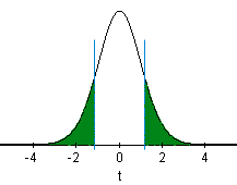
Find the \(P\)-value and compare it to the level of significance

\[P\text{-value}=0.2295 > 0.05 = \alpha\]

State your decision

Since the \(P\)-value is greater than the level of significance, we fail to reject the null hypothesis.

Present your conclusion in an easy to understand sentence, relating the result to the context of the problem

There is insufficient evidence to suggest that the mean weight of babies born in Australia is different from 3373 grams.

Confidence Intervals

The procedure for finding confidence intervals when \(\sigma\) is not known is very similar to the process when \(\sigma\) is known. As a reminder, here is the confidence interval (from Lesson 10) when \(\sigma\) is known. \[ \left( \bar x - z^* \frac{\sigma}{\sqrt{n}}, ~ \bar x + z^* \frac{\sigma}{\sqrt{n}} \right) \]

To construct the confidence interval when \(\sigma\) is not known, we replace the population standard deviation, \(\sigma\), with its point estimate, \(s\). The appropriate distribution is a \(t\), rather than a \(z\). So, we replace \(z^*\) with \(t^*\). So the confidence interval when \(\sigma\) is not known is \[ \left( \bar x - t^* \frac{s}{\sqrt{n}}, ~ \bar x + t^* \frac{s}{\sqrt{n}} \right) \] where \(t^*\) is the \(t\)-score corresponding to the confidence level and \(s\) is the sample standard deviation.

We will use Excel to construct confidence intervals when \(\sigma\) is unknown. The values of \(t^*\) and \(s\) will be computed for us. Examples of this are given below. You can see the details by clicking on [Show Hand Calculations] in Step 4.

Automatic Language Translation Programs

Summarize the relevant background information

Computer software is commonly used to translate text from one language to another. As part of his Ph.D. thesis, Philipp Koehn developed a phrase-based translation program called Pharaoh.

The quality of the translation can vary. A good translation system should match a professional human translation. It is important to be able to quantify how good the translations produced by Pharaoh are.

The IBM T. J. Watson Research Center developed methods to measure the quality of a translation from one language to another. One of these is the BiLingual Evaluation Understudy (BLEU). BLEU is a score ranging from 0 to 1 that indicates how well a computer translation matches a professional human translation of the same text. Higher scores indicate a better match. BLEU helps companies who develop translation software “to monitor the effect of daily changes to their systems in order to weed out bad ideas from good ideas”.

Describe the data collection procedures

To test Pharaoh’s ability to translate, Koehn took a random sample of 100 blocks of Spanish text, each of which contained 300 sentences, and used Pharaoh to translate each of these to English. The BLEU score was calculated for each of the 100 blocks. The data were extracted from Figure 2 in a paper Koehn published. The 100 BLEU scores are given in BLEU-Scores.

Koehn wants to find an estimate of the true mean BLEU score for text translated by the Pharaoh computer program. He would like to compute a confidence interval, but he does not know the true population standard deviation, \(\sigma\).

Give the relevant summary statistics

Excel Instructions

Copying the BLEU-Scores data into the Math 221 Statistics Toolbox file in Excel, we get the following:

The summary statistics are:

\[ \begin{align} \bar x =& 0.288 \\ s =& 0.026 \\ n =& 100 \end{align} \]

Make an appropriate graph to illustrate the data

The histogram is included in the image above.

Make Inference

Find the confidence interval

We will use Excel to find the confidence intervals for the mean.

Excel Instructions

Do the following:

• Open the file Math 221 Statistics Toolbox
• Click on the tab labeled “One-sample t-test”
• Enter the data, and
• Set the confidence level.

In this case, we are using a 95% confidence level. So, you set the confidence level in the Excel file to 0.95 (i.e., 95%). The confidence interval is given to you in cells L14 and M14.

The 95% confidence interval for the true mean BLEU score is:

\[(0.282, 0.293)\]

Show Hand Calculations

The formula for the confidence interval where \(\sigma\) is known was given in the reading titled Lesson 10: Inference for One Mean: Sigma Known (Confidence Interval) as \[ \left( \bar x - z^* \frac{\sigma}{\sqrt{n}}, ~ \bar x + z^* \frac{\sigma}{\sqrt{n}} \right) \] It is impossible to know the true standard deviation of the BLEU scores for a new translation program like Pharaoh. Replacing \(\sigma\) with \(s\) and replacing \(z^*\) with \(t^*\), we get: \[ \left( \bar x - t^* \frac{s}{\sqrt{n}}, ~ \bar x + t^* \frac{s}{\sqrt{n}} \right) \] The value of \(t^*\) depends on the level of confidence and the sample size. It must be computed using software or looked up on a table. If you are asked to compute a confidence interval for a mean where the population standard deviation is unknown, the value of \(t^*\) will be given to you. The other numbers (\(\bar x\), \(s\), and \(n\)) can all be obtained directly from your data.

If we want to create a 95% confidence interval for \(\mu\), with 99 degrees of freedom, then \(t^* = 1.9842\).

Using the sample statistics: \[ \begin{align} \bar x =& 0.2876 \\ s =& 0.0264 \\ n =& 100 \end{align} \]

The 95% confidence interval for \(\mu\) is: \[ \left( 0.2876 - 1.9842 \frac{0.0264}{\sqrt{100}}, ~ 0.2876 + 1.9842 \frac{0.0264}{\sqrt{100}} \right) \] which reduces to: \[ \left( 0.2824, ~ 0.2928 \right) \]

Verify Requirements Are Met

The requirements for creating a confidence interval for a mean with \(\sigma\) unknown are the same as the requirements for this procedure when \(\sigma\) is known:

There are two requirements that need to be checked:

1. A simple random sample was drawn from the population
2. \(\bar x\) is normally distributed

Recall the requirement of normality is satisfied if the data are approximately normally distributed or if the sample size is large.

The data are bell-shaped and fairly symmetric. So, the sample mean, \(\bar x\), is approximately normally distributed.

Present your observations in an easy to understand sentence, relating the result to the context of the problem

We are 95% confident that the true mean BLEU score for all translations by the Pharaoh program is between 0.2824 and 0.2928.

Answer the following questions using the data set BLEU-Scores, which gives the BLEU scores for \(n=100\) translations from Spanish to English by the computer program Pharaoh.

Answer the following questions:

5. Use Excel to find a 90% confidence interval for the true mean BLEU score for translations by the Pharaoh program. Give your answer accurate to 3 decimal places. Interpret this confidence interval in a complete sentence.

Show/Hide Solution

• \((0.283, 0.292)\)
  We are 90% confident that the true mean BLEU score for translations by the Pharaoh program lies between 0.283 and 0.292.

6. Use Excel to find a 99% confidence interval for the true mean BLEU score for translations by the Pharaoh program. Give your answer accurate to 3 decimal places. Interpret this confidence interval in a complete sentence.

Show/Hide Solution

• \((0.281, 0.295)\)
  We are 99% confident that the true mean BLEU score for translations by the Pharaoh program lies between 0.281 and 0.295.

7. What do you notice about the confidence interval as the confidence level increased from 90% to 99%?

Show/Hide Solution

• As the confidence level increases, the width of the confidence interval increases. We could also say, as the confidence level increases, the margin of error increases. The center of the confidence interval (the sample mean) is unchanged.

 

Euro Weights

Summarize the relevant background information

A group of statisticians measured the weights of 2000 Belgian one Euro coins in eight batches. Each batch contains coins that were all minted together. You can learn more about these data at: http://www.amstat.org/publications/jse/

Describe the data collection procedures

The coins were “borrowed” from a bank in Belgium, one batch at a time. The weights (in grams) of the coins are given in the file EuroWeight.xlsx.

Answer the following questions:

8. Give the relevant summary statistics.

Show/Hide Solution

The following output was generated using the Excel file Math 221 Statistics Toolbox:

• Typically, we round our computations to one more decimal place of precision than was given in the original data. This means we need one more decimal place than is shown in the output above. We can increase the precision by selecting the cell we want to modify and then clicking on the following button in the “Home” menu ribbon in Excel:

• When we do this, we get the following summary statistics:

\[ \begin{align} \bar x =& 7.521 \\ s =& 0.0344 \\ n =& 2000 \end{align} \]

9. Make an appropriate graph to illustrate the data

CAUTION: The Excel Toolbox boxplot only works for datasets of 1,000 observations or less. This dataset contains 2,000 observations. You will need to create your own boxplot.

Show/Hide Solution

If you create your own histogram and boxplot of the data, the graphs should look something like the image below

You can see the data is relatively normal, with just a couple of potential outliers that could be investigated further.

 

Verify the requirements have been met

We need to check the following two requirements:

1. A simple random sample was drawn from the population
2. \(\bar x\) is normally distributed

The coins were taken in batches, but we can think of the batches as a random sample of the possible coins that could be chosen.

The data follow a bell-shaped distribution. There are a few potential outliers, but they are not too frequent or extreme. We can conclude that \(\bar x\) is normally distributed.

Answer the following question:

10. Find the confidence interval: Use Excel to create a 99% confidence interval for the true mean.

Show/Hide Solution

\[ (7.519, ~ 7.523) \]

 

Answer the following questions:

11. Present your observations in an easy to understand sentence, relating the result to the context of the problem.

Show/Hide Solution

• We are 99% confident that the true mean weight of all Belgian Euros is between 7.519 grams and 7.523 grams.

 

Summary

Remember…

• In practice we rarely know the true standard deviation \(\sigma\) and will therefore be unable to calculate a z-score. Student’s t-distribution gives us a new test statistic, \(t\), that is calculated using the sample standard deviation (\(s\)) instead. \[\displaystyle{ t = \frac {\bar x - \mu} {s / \sqrt{n}} }\]

• The \(t\)-distribution is similar to a normal distribution in that it is bell-shaped and symmetrical, but the exact shape of the \(t\)-distribution depends on the degrees of freedom (\(df\)). \[df=n-1\]

*You will use Excel to carry out hypothesis testing and create confidence intervals involving \(t\)-distributions.

Navigation

Previous Reading	This Reading	Next Reading
Lesson 10: Inference for One Mean: Sigma Known (Confidence Interval)	Lesson 11: Inference for One Mean: Sigma Unknown	Lesson 12: Inference for Two Means: Paired Data

---

Copyright © 2020 Brigham Young University-Idaho. All rights reserved.