Lesson 12: Inference for the Mean of Differences (Two Dependent Samples)

Optional Videos for this Lesson

Part 1

Part 2

Part 3

Lesson Outcomes

By the end of this lesson, you should be able to do the following:

1. Recognize when a mean of differences (two dependent samples) inferential procedure is appropriate
2. Create numerical and graphical summaries of the data
3. Perform a hypothesis test for the mean of differences (two dependent samples) using the following steps:
   1. State the null and alternative hypotheses
   2. Calculate the test-statistic, degrees of freedom and P-value of the test using software
   3. Assess statistical significance in order to state the appropriate conclusion for the hypothesis test
   4. Check the requirements for the hypothesis test
4. Create a confidence interval for the mean of differences (two dependent samples) using the following steps:
   1. Calculate a confidence interval using software
   2. Interpret the confidence interval
   3. Check the requirements of the confidence interval

Example of Paired Data: Pre- and Post-test Scores

In education, it is very common for researchers to conduct studies in which they administer a pre-test, provide some instruction, and then give a post-test. The difference between the post- and pre-test scores is a measure of the student’s progress. In this case, it would not make much sense to only look at the mean score on the pre-test and compare it to the mean score on the post-test.

This is called a matched-pairs design or we say we have dependent samples. Matched-pairs (or paired-data) designs typically involve only one population, and a pair of observations is drawn on the individuals selected for the sample. In the context of the educational study, the two observations are student’s scores on (1) the pre-test and (2) the post-test. If a student is selected to participate in the pre-test (i.e., they are selected to be part of group 1), they are automatically selected to participate in the post-test (i.e., they are chosen to be in group 2 automatically.)

There is a lot of merit in subtracting the individual scores and looking at the mean gain. The researchers are not really interested in the students knowledge before the instruction. This is used as a baseline to measure how much was gained during the instruction. There is great value in looking at the difference. This removes the effect of the individual students’ ability, and it measures their learning during the unit.

To analyze the data, the researchers first find the difference in the post- and pre-test scores. At that point, the data have been reduced to a list of numbers (representing the increase in scores). Now, the researchers can conduct inference on the mean of these values. In other words, they can do a hypothesis test for the mean of the difference in the post- and pre-test scores.

A hypothesis test for two means with paired data (dependent samples) is conducted in the same way as a hypothesis test for a single mean with \(\sigma\) unknown. The only exception is that the pairs of data must be subtracted before you start any computations. From a practical perspective, after you subtract, then you apply the one-sample procedures you have already learned. So, there is nothing new that you need to learn to compute a confidence interval for two means with paired data; just that we will be using a different sheet in the Math221 Statistics Toolbox that automatically calculates the differences.

We will first explore an application of pre- and post-testing in a weight loss study.

Hypothesis Tests

Mahon’s Weight Loss Study

Background

Annie Mahon and other researchers in Wayne Campbell’s nutrition lab studied the weight loss of \(n=27\) middle aged women who consumed a prescribed low-calorie diet. The women’s weights were recorded (in kilograms) at the beginning of the study and after the nine-week diet period. The data are given in the file Mahon.xlsx. An excerpt of the data is given below.

Subject	Pre	Post
1	62.5	56.1
2	88.8	80.2
3	74.7	70.8
\(\vdots\)	\(\vdots\)	\(\vdots\)
26	76.3	73.8
27	82.1	77.9

Notice the structure of the data. The weight of each subject was measured before the study and at the conclusion of the study. Each person provided a pre-study weight and a post-study weight. Stated differently, the pre-study weights and the post-study weights are paired. For each row of data, both of these numbers came from the same person. When we collect two observations of the same measurement on each subject, we call it paired data. Sometimes paired data are called dependent samples.

Answer the following question:

1. The researchers measured the initial weights of the women prior to the study, even though they were not particularly interested in this value. What was the purpose of measuring the pre-study weights?

Show/Hide Solution

• The goal of the study is to determine how much the women’s weight change as as result of the study. The researchers must measure the women’s weights at the beginning of the study, so they can subtract the initial (pre-study) weight of each woman from her final (post-study) weight.

 

Computing New Variables in Excel

The researchers are not interested in the weights of the women, they are more interested in the change in the women’s weights. This will give them a measure of the effectiveness of the low-calorie diet. In other words, they are interested in the difference of the weights after the study compared with before: \[\text{Difference} = \text{Post} - \text{Pre}\]

We can calculate the difference for each woman in the study:

Subject	Post	Pre	Difference
1	56.1	62.5	56.1 \(-\) 62.5 = -6.4
2	80.2	88.8	80.2 \(-\) 88.8 = -8.6
3	70.8	74.7	70.8 \(-\) 74.7 = -3.9
\(\vdots\)	\(\vdots\)	\(\vdots\)	\(\vdots\)
26	73.8	76.3	73.8 \(-\) 76.3 = -2.5
27	77.9	82.1	77.9 \(-\) 82.1 = -4.2

Excel Instructions

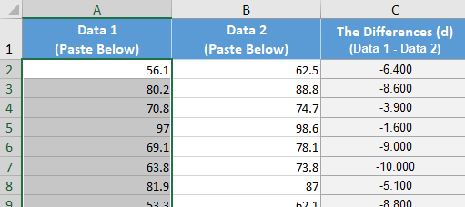
Fortunately, the “Paired Data t-test” tab in the Math 221 Statistics Toolbox will automatically compute the differences when you paste in the data. The Toolbox always takes the data in column A - data in column B. Because we want to take Post - Pre, you will need to swap the order of the columns when pasting the data into the Math221 Statistics Toolbox. Follow this process:

• Copy the “Pre” column and paste it into column B, labeled “Data2” of the Toolbox.
• Copy the “Post” column and paste it into column A, labeled “Data1” of the Toolbox.
• Notice in column C the differences are automatically calculated.
• A excerpt of how the data looks in the Math221 Statistics Toolbox is shown below:

Answer the following questions:

2. Following the directions above, compute the difference in the women’s weights by pasting the data in the Math221 Statistics Toolbox.

3. What is the mean of the values in the Difference column? (Look in cell G7)

Show/Hide Solution

\[ -6.80 \text{ kg} \]

4. Interpret the value you calculated in Question 3.

Show/Hide Solution

• The mean weight change experienced by the women in the study was \(-6.80\) kg. It can be tricky to know if this means they gained or lost weight. Remember, we calculated Post-Pre. A negative difference indicates the Pre weight was higher than the Post weight. In other words, there was a mean weight loss of \(6.80\) kg.

 

Relationship to a One Sample t-test

After you have subtracted the pre-study weights from the post-study weights, you are left with a column of differences. We will denote the pre-study weights by \(x_1\) and the post-study weights by \(x_2\). Then, the differences can be denoted as \(d = x_2 - x_1\). The difference, \(d\), is defined as the change in the volunteer’s weight during the study.

After computing the differences, we do not use the data for the individual groups at all. The researchers are not interested in the values of the women’s weights at the beginning of the study or at the end of the study. They are mostly interested in the difference in the weights after the participants complete the study.

After we subtract, we can conduct a hypothesis test to determine if the mean of the differences is less than zero. We use the symbol \(\mu_d\) to represent the true mean difference in the weights of the women who follow the diet prescribed in this study. The null hypotheses is that the true mean difference is zero (\(\mu_d = 0\)). The alternative hypothesis is that there is a decrease in the weights, in other words, that the true mean difference is less than zero (\(\mu_d < 0\)).

Notice that this is essentially a one-sample t-test where the data are the differences in the women’s weights. We have one column of data, the differences. We are testing whether the true mean difference is less than zero. After subtracting, a test for a difference of two means with paired data is just like a test for one mean with \(\sigma\) unknown.

In the hypothesis test, we will refer to the variable representing the differences as \(d\). We will use this notation throughout the hypothesis test. For example, the true population mean will be labeled \(\mu_d\) and the sample mean will be labeled \(\bar d\). The sample standard deviation of the differences is denoted \(s_d\).

Hypothesis Test for Mahon’s Weight Loss Data

Summarize the relevant background information

Twenty-seven women participated in a nine week weight loss study. During the study period, the participants were provided a reduced calorie diet. Their weights were recorded at the beginning of the study and nine weeks later. The difference of the weights is defined as the post-study weights minus the pre-study weights. The researchers expected that the mean difference in the weights would be negative–in other words, that the women would tend to lose weight.

State the null and alternative hypotheses and the level of significance

\[ \begin{align} H_0: &~~ \mu_d=0 \\ H_a: &~~ \mu_d < 0 \end{align} \]

We will use the \(\alpha = 0.05\) level of significance.

Describe the data collection procedures

The women’s weights were recorded at the beginning of the study. The women were provided a reduced calorie diet for nine weeks. Then, their weights were measured again at the end of the study. A calibrated scale was used to provide an accurate weight.

Give the relevant summary statistics

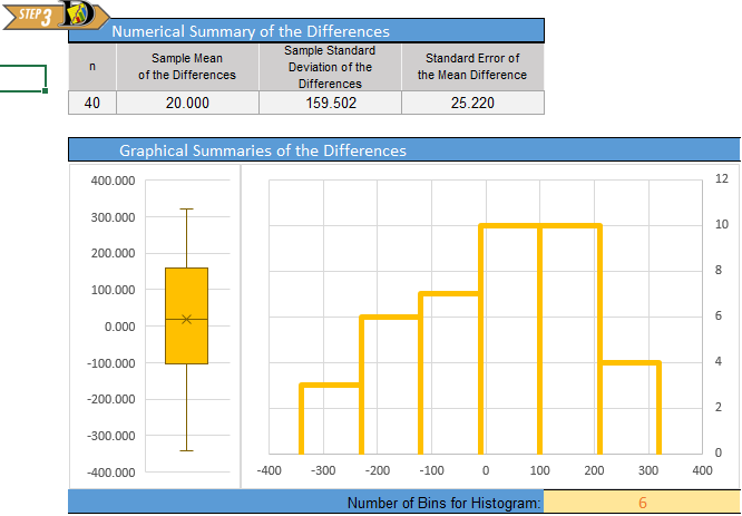
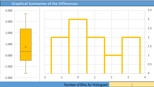
Here is the Excel output:

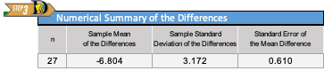
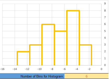
From the Excel output illustrated above, we can see a histogram of the data and get the following numerical summaries:

\[ \begin{align} \bar d &= -6.80 \\ s_d &= 3.17 \\ n &= 27 \end{align} \]

The mean and standard deviation are rounded to one decimal place more than the original data.

Verify the requirements have been met

Like the one-sample t-test, this procedure is robust, meaning that it is not very sensitive to the requirements. If they are violated, it will probably still give reasonably good results.

The requirements for this procedure are the same as the requirements for a one-sample t-test:

• the data represent a simple random sample from the population
• the mean of the differences follows a normal distribution

The subjects were recruited via advertisements for a research study. The participants volunteered to participate. It is not a simple random sample of all middle-aged women, but there is nothing about the selection of the sample that would invalidate the results.

From a practical perspective, it is impossible to get a simple random sample of people in the general population. When research trials are conducted, people must volunteer to participate. This can lead to a selection bias, but it is usually negligible.

The requirement of normality is satisfied for Mahon’s data. Though the sample size (n=27) is not quite up to 30, it is still fairly large. Furthermore, the histogram of differences indicates very little skew, so \(\bar d\) will be approximately normal.

Even with a sample size less than 30, we can still conduct this test.

Give the test statistic and its value

The test statistic for a test involving paired data when \(\sigma\) is unknown is a \(t\). For this situation, the value is: \[t= \frac{-6.8 - 0}{3.17/\sqrt{27}} =-11.145\] See that this calculation matches the test statistic given in the Excel output. The degrees of freedom and p-value can also be found in the Excel output.

State the degrees of freedom

\[df = 26\]

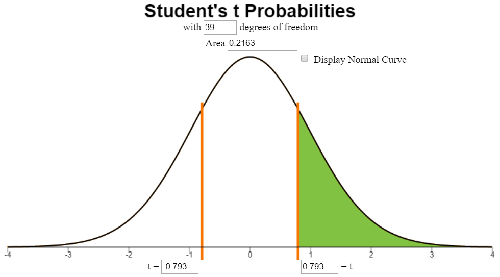
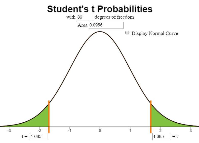
Mark the test statistic and \(P\)-value on a graph of the sampling distribution

The test statistic and p-value can be found in the Excel output. The following calculations show conceptually how the p-value is calculated:

The test statistic, \(t\), is labeled on the horizontal axis. The \(P\)-value is the area to the left of \(t\) under the curve. This area is so small, it is hiding out on the edges (not actuall visible) on this plot.

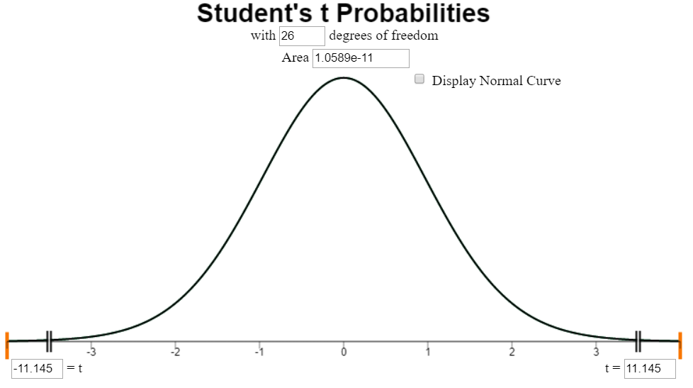
It is important to note that only the left tail is shaded, even though we cannot see it in this illustration.

Find the \(P\)-value and compare it to the level of significance

\[ P\text{-value} = 1.06 \times 10^{-11} < 0.05 = \alpha \]

State your decision

Since the \(P\)-value is less than the level of significance, we reject the null hypothesis.

Present your conclusion in an English sentence, relating the result to the context of the problem

There is sufficient evidence to suggest that the reduced calorie diet used in this study results in weight loss for middle-aged women.

Nosocomial Infections

Summarize the relevant background information

Matched-pairs designs are not just used in pre- and post-test situations. They are often used in situations where it is not possible to randomly assign subjects to groups (for example, by a coin toss.) Nosocomial (pronounced: NO-suh-KOH-MEE-uhl) infections are infections that occur in hospitals, but are not a result of the original condition. An example of a nosocomial infection is when a heart attack patient develops a staph infection at the site of an IV injection. The infection was not caused by the heart attack, but it was acquired in the hospital. Nosocomial infections are very dangerous and may result in longer recovery times or increased death rates.

Health care providers suspect that nosocomial infections increase the amount of time required to recover from an illness or injury. In controlled experiments, subjects (e.g., patients) are randomly assigned to treatments. However, it is not ethical to give patients a nosocomial infection in order to determine if it increases the duration of their hospital stay! At best, we can collect information on the duration of hospital stays for patients who acquire nosocomial infections and compare them to the duration of the stays for patients who do not.

There are many factors that affect the amount of time that a patient will need to stay in the hospital, including: nature of illness, types of procedures conducted, overall health, gender, age, etc. How can health care practitioners assess the effect of a nosocomial infection in the presence of so many other variables?

One way is to match a patient who develops a nosocomial infection with another one who has similar characteristics (illness, procedures, health, gender, age group, etc.) but does not develop a nosocomial infection. Now, the patients are matched into pairs with similar characteristics, where the principle difference between the members of each pair is whether or not they acquired a nosocomial infection.

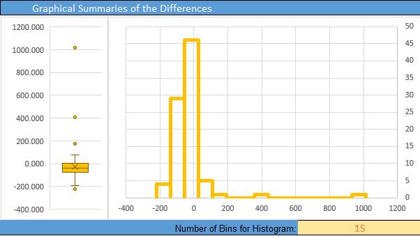
By pairing the patients according to specific characteristics, the researchers can now subtract to observe a difference in their recovery times. In this way, it is possible to assess if nosocomial infections increase the mean duration of a hospital stay. Some researchers conducted such a study in which 52 pairs of patients were matched based on clinical characteristics. A patient with a nosocomial infection was matched as closely as possible to a similar case where there was no nosocomial infection. Patients who died were excluded from the study . The lengths of the hospital stays (in days) for these patients are given in the file NosocomialInfections.xlsx.

The difference, \(d\), is defined as the duration of the hospital stay of the individual in the pair with the nosocomial infection minus the duration of the stay for the individual who did not get a nosocomial infection: \[ Difference=Infected - NotInfected \] After computing the differences, we do not use the data for the individual groups at all. In fact, after we subtract, the hypothesis test is conducted (essentially) like a one-sample test for a single mean with \(\sigma\) unknown.

Answer the following questions:

5. State the null and alternative hypotheses and the level of significance

Show/Hide Solution

\[ \begin{align} H_0: &~~ \mu_d = 0 \\ H_a: &~~ \mu_d > 0 \\ \end{align} \]

• The level of significance was not specified in the problem. You can choose any value you wish. The most common choices are 0.05, 0.01 and 0.1. We will illustrate this example with \(\alpha = 0.05\).

 

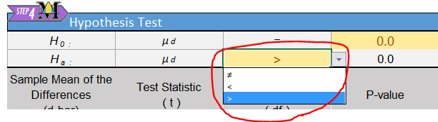
In order to get the correct \(P\)-value, we need to indicate the proper alternative hypothesis in Excel. In cell N6 be sure the “Greater Than” symbol is selected in the drop-down menu.

Answer the following questions:

6. Describe the data collection procedures

Show/Hide Solution

• Data were collected by matching hospital records of individuals who were admitted to the hospital. Patient records were matched based on their overall health and the reason they were admitted to the hospital. In each pair, one patient developed a nosocomial infection and one did not. Since the characteristics of the patients in the first group determined which patients would be paired with them in the second group, the data represent dependent samples.

 

Answer the following questions:

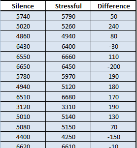
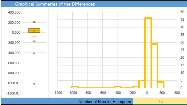
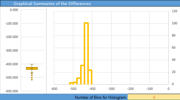
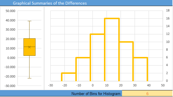
7. Give the relevant summary statistics

Show/Hide Solution

\[ \begin{align} \bar d &= 11.38 \\ s_d &= 13.83 \\ n &= 52 \end{align} \]

8. Make an appropriate graph to illustrate the data

Show/Hide Solution

• Present a graph showing the differences.

 

Answer the following questions:

9. Verify the requirements have been met

Show/Hide Solution

• The data represent a random sample of patients, who have been matched based on their overall health and their current ailment. The sample size is large, so the mean of the differences \(\bar d\) will be approximately normally distributed.

10. Give the test statistic and its value

Show/Hide Solution

• The test statistic for a test for two means with paired data is a \(t\).

\[t = 5.935\]

11. State the degrees of freedom

Show/Hide Solution

\[ df = 51 \]

12. Mark the test statistic and \(P\)-value on a graph of the sampling distribution

Show/Hide Solution

• The test statistic and p-value can be found in the Excel output and you should not need to calculate it by hand. Your sketch should show the value of \(t=5.935\) on the horizontal axis, with only the tiny area to the right of 5.935 shaded.

13. Find the \(P\)-value and compare it to the level of significance

Show/Hide Solution

The p-value can be found in the Excel output and you should not need to calculate it by hand. The calculation below shows how the p-value in Excel is being calculated: \[ P\textrm{-value}=\frac{\textrm{Sig. (2-tailed)}}{2}=\frac{2.592\times 10^{-7}}{2}=1.296 \times 16^{-7} = 0.0000001296 < 0.05 = \alpha \]

14. State your decision

Show/Hide Solution

• Since the \(P\)-value is less than the level of significance, we reject the null hypothesis.

 

Answer the following questions:

15. Present your conclusion in an English sentence, relating the result to the context of the problem

Show/Hide Solution

• There is sufficient evidence to suggest that the mean duration of hospital stays is increased when a patient develops a nosocomial infection.

 

Additional Worked Examples

Viewing additional examples can help your understanding. Click on the link below to see two more examples of hypothesis tests.

Show/Hide Additional Examples

Effect of Stressful Classical Music on Your Metabolism

Summarize the relevant background information

Obesity is a growing problem worldwide. Many scientists are seeking creative solutions to trim down this epidemic. Reduced energy expenditure is a potential cause of obesity.

Resting Energy Expenditure (REE) is defined as the amount of energy a person would use if resting for 24 hours. In essence, this is the amount of energy that a person’s body will consume if they do not do any physical activity. REE is measured in terms of kilo-Joules per day (kJ/d).

REE accounts for approximately 70 to 80% of all energy that a person will expend in a day. If researchers can find simple, enjoyable activities that will increase REE, it may be possible to minimize the spread of obesity around the world.

Ebba Carlsson and other researchers in Sweden investigated whether listening to stressful classical music increases a person’s REE. Each subject’s REE was measuring during silence and again while listening to stressful classical music. Data representing their results are given in the file REE-ClassicalMusic.

Notice that this is not a pre- and post-test, but it is still a test involving paired data. Two REE measurements were made for each subject: (1) in silence (\(REE_1\)) and (2) while listening to stressful classical music (\(REE_2\)).

State the null and alternative hypotheses and the level of significance

Since we are testing for an increase in the mean REE, we let \(d = REE_2 - REE_1\). Our alternative hypothesis will be that \(\mu_d > 0\). The null and alternative hypotheses are: \[ \begin{align} H_0: &~~ \mu_d = 0 \\ H_a: &~~ \mu_d > 0 \end{align} \]

Note that the data set has the columns listed with \(d = REE_1\) in the first column and \(d = REE_2\) in the second column. You will need to switch the order of the columns when pasting them into the Excel Toolbox.

We will use the \(\alpha = 0.1\) level of significance.

Describe the data collection procedures

The REE was measured by a technique called “indirect calorimetry” using a Deltatrac II Metabolic Monitor. The REE was measured twice for each person: while the person was (1) resting in silence or (2) resting while listening to stressful classical music. These trials were conducted in random order. Some of the subjects had the “silence” treatment first, and others had the “stressful” treatment first.

Answer the following questions:

16. We will define the difference in REE by subtracting the REE in silence from the REE while listening to stressful classical music. If listening to stressful classical music actually increases the mean REE, would you expect the value of the difference to be typically positive or negative?

Show/Hide Solution

• If the REE is higher while listening to classical music than while resting in silence, we would expect the value of the difference to be positive. In other words the following difference would tend to be positive:

\[ Difference = Stressful - Silence \]

17. Compute the difference in REE for each person. What is the value of the difference for the first person listed in the data file?

Show/Hide Solution

• 50 kJ/d

• Here is an illustration of an excerpt of the data in Excel:

  

Give the relevant summary statistics

18. Report the number of subjects (\(n\)), the mean difference (\(\bar d\)), and the standard deviation of the differences (\(s_d\)).

Show/Hide Solution

The following image illustrates the Excel file used to get the summary statistics.

\[ \begin{align} n&=40\\ \bar d &= 20~\text{kJ}\\ s_d &= 160~\text{kJ} \end{align} \]

19. See above output for a graph of the data

Verify the requirements have been met

We can consider the sample representative of the population. Because our sample size (n=40) of differences is greater than 30, we can be sure the sampling distribution of \(\bar d\) will be normal.

The requirements for this test appear to have been satisfied.

Answer the following questions:

20. Give the test statistic and its value

Show/Hide Solution

• The test statistic for a test for two means with paired data is a \(t\).

\[t=0.793\]

21. State the degrees of freedom

Show/Hide Solution

\[ df = 39 \]

22. Mark the test statistic and \(P\)-value on a graph of the sampling distribution

Show/Hide Solution

• The test statistic is plotted on the horizontal axis. The \(P\)-value is shaded in green. The same value can be found on the Excel output in cell O10.

23. Find the \(P\)-value and compare it to the level of significance

Show/Hide Solution

\(P\textrm{-value}=0.2163 > 0.1 = \alpha\)

• Notice that the \(P\)-value is half as large for a one-tailed test as it would have been for a two-tailed test. Since we have a one-sided alternative hypothesis, we are only interested in the right tail of the \(t\)-distribution.

24. State your decision

Show/Hide Solution

• Since the \(P\)-value is greater than the level of significance, we fail to reject the null hypothesis.

 

Answer the following questions:

25. Present your conclusion in an English sentence, relating the result to the context of the problem

Show/Hide Solution

• There is insufficient evidence to suggest that the mean REE is increased by listening to stressful classical music. Lying still and listening to stressful classical music is probably not the best way to increase your metabolism!

 

Note that we did not say we “accept” the null hypothesis. We do not know that listening to stressful classical music has no effect on a person’s REE. Based on the data available to us, we were not able to reject the assertion that this type of music does not increase the mean REE.  

Cost of Airline Tickets

Summarize the relevant background information

Pressures of supply and demand act directly on the prices for an airline ticket. As the seats available on the plane begin to fill, airlines raise the price. If seats on a flight do not sell well, an airline may discount the tickets or even cancel the flight. Business travelers frequently demand travel booked on short notice. They must pay the current price. Typically, tourists book their flights well in advance, hoping to buy tickets before the price rises. We will consider the cost of a one-way ticket from London’s Heathrow Airport to a variety of destinations in Europe.

Allie Henrich, a BYU-Idaho student, compared the lowest published ticket prices of one-way flights from Heathrow to various destinations in Europe. Using Travelocity.com, she recorded the lowest published fares for nonstop midweek flights booked either 14 days in advance or 90 days in advance. The prices (in US dollars) are given in the file DirectFlightCosts.xlsx. Notice that for some destinations, flights were not available.

The data are paired, because we are measuring the costs twice for each city. The 14-day ticket price is paired with the 90-day price for each city.

We will conduct a hypothesis test to determine if there is a difference in the cost of the nonstop flights when tickets are purchased 14 days in advance compared to 90 days in advance. We will use the 0.01 level of significance.

Answer the following questions:

26. State the null and alternative hypotheses and the level of significance

Show/Hide Solution

\[ \begin{array}{1cl} H_0:\mu_d = 0 \\ H_a:\mu_d \ne 0 \\ \alpha = 0.01 \end{array} \]

 

Answer the following questions:

27. Describe the data collection procedures

Show/Hide Solution

• The data were collected using the website Travelocity.com. The lowest advertized ticket prices were recorded for nonstop flights from Heathrow Airport. All prices were recorded in US dollars. Data are provided on the cost of a nonstop ticket purchased with 14 days notice compared to 90 days notice.
• We will compute the difference in the costs for each destination. Some destinations did not include both flight options. In this case, the difference is not computed and the data are omitted from the analysis.

 

Answer the following questions:

28. Give the relevant summary statistics

Show/Hide Solution

• The differences were computed by subtracting the 90-day price from the 14-day price. For example, for the Adnan Menderes Airport, we have

\[202.09 - 234.19 = -32.10\]

• You may have chosen to subtract in the opposite order. If so, you would have obtained a value of \(32.10\) dollars.

\[ \begin{align} n&=87\\ \bar d &= 24.612\\ s_d &= 136.267 \end{align} \]

If you defined your difference as the 90-day price minus the 14-day price, then you would have observed a value of \(\bar d = -24.612\) dollars for the mean of the differences. You were not instructed on the order in which to subtract, so this is a correct response. The value for the standard deviation of the difference and the number of observations (pairs) will be the same as is given above.

29. Make an appropriate graph to illustrate the data

Show/Hide Solution

• If you defined your difference as the 90-day price minus the 14-day price, then you would have the following histogram:

 

Answer the following questions:

30. Verify the requirements have been met

Show/Hide Solution

• The sample size is large, so we can conclude that the sample mean, \(\bar d\) is normally distributed.

31. Give the test statistic and its value

Show/Hide Solution

• The test statistic for a test for two means with paired data is a \(t\).

\[t=1.685\]

• If you computed the difference as the 90-day price minus the 14-day price, the value of your test statistic is \(-1.685\).

32. State the degrees of freedom

Show/Hide Solution

\[ df = 86 \]

33. Mark the test statistic and \(P\)-value on a graph of the sampling distribution

Show/Hide Solution

• The test statistic is plotted on the horizontal axis. The \(P\)-value is shaded in green:

34. Find the \(P\)-value and compare it to the level of significance

Show/Hide Solution

\[ P\textrm{-value}= 0.096 > 0.01 = \alpha \]

The \(P\)-value will be 0.096, no matter what order you subtracted the values.

35. State your decision

Show/Hide Solution

Since the \(P\)-value is greater than the level of significance, we fail to reject the null hypothesis.

 

Answer the following questions:

36. Present your conclusion in an English sentence, relating the result to the context of the problem

Show/Hide Solution

• There is insufficient evidence to suggest that there is a difference in the mean cost of airline tickets 14-days versus 90-days in advance.

 

Confidence Intervals

We can compute a confidence interval for the true mean of the differences for paired data. After the differences between two paired data sets have been calculated, we can create a confidence interval for the true mean of the differences. To do this, we follow the instructions for creating a confidence interval for a one mean with \(\sigma\) unknown, but we use the column of differences as the data set.

Excel Instructions

To calculate confidence intervals for the true mean of the difference in Excel, do the following:

• Open the file Math 221 Statistics Toolbox
• Click on the tab labeled “Paired Data t-test”
• Enter the columns of paired data into column A and B
• Set the desired confidence level.
  

The requirements for creating a confidence interval for the difference of means are the same as the requirements for the hypothesis test. We assume:

• A simple random sample was drawn from the population
• The mean of the differences is normally distributed

 

Mountain Pine Beetle Attacks

Summarize the relevant background information

Mountain pine beetles are small insects that bore into the bark of trees. The female beetles that first infest the tree emit pheromones to attract other beetles. In response to the pheromones, many beetles bore into the tree and ultimately kill it. The insects can destroy large tree stands within one year.

Lodgepole pine (Pinus contorta Dougl.ex Loud.) are particularly susceptible to mountain pine beetle (Dendroctonus ponderosae Hopkins) outbreaks. The image above shows the destruction that can be caused by these insects. The large brown patches are pines that have been killed by the beetles.

Answer the following questions:

37. The mountain pine beetle threatens many forests in the United States. These tiny insects are only 0.5 cm long–about the size of a grain of rice. This photo of a mountain pine beetle is magnified greatly. These little creatures can destroy a large, healthy forest. Can you think of a spiritual parallel?

Show/Hide Solution

• There are many great diverse answers that could be presented. Please share your thoughts with someone in your group.

 

Describe the data collection procedures

In a study conducted in the Arapaho National Forest in Colorado, researchers from the USDA Forest Service studied the effect of pine beetle outbreaks on the average number of trees in an area. The researchers counted the number of established trees per hectare before a pine beetle outbreak and seven years after an outbreak. (One hectare is an area of 100 meters by 100 meters.) Data representative of their observations are given in the file PineBeetle.xlsx.

Answer the following questions:

Give the relevant summary statistics

38. Find the mean and standard deviation of the number of trees per hectare before the pine beetle outbreak. How would you describe the density of the trees in this forest? Express this in terms that make sense to you.

Show/Hide Solution

• The mean was 1028.41 trees per hectare and the standard deviation was 57.03 trees per hectare. Note that the values were rounded to two decimal places, since the data were given to one decimal place.
• Answers will vary regarding the description of the density. Here is one possible response.
• There is roughly one tree every \(\frac{100 \times 100}{1028.41} = 9.7\) square meters. In other words, on average, each tree would have a space of about \(\sqrt{9.7} = 3.1\) meters long and 3.1 meters wide in which to grow.

39. Repeat question 38 for the number of trees per hectare after the outbreak.

Show/Hide Solution

• The mean was 592.87 trees per hectare and the standard deviation was 45.31 trees per hectare.
• Answers will vary regarding the description of the density. Here is one possible response.
• The trees are about half as dense as they were before the pine beetle infestation. About \(\frac{592.87}{1028.41} = 0.58 = 58\%\) of the trees remained, so \(100\% - 58\% = 42\%\) of the trees were killed by the pine beetles!

40. Find the differences by subtracting the “before” counts from the “after” counts:

\[Difference = After - Before\] You will need to change the order of the columns so that “after” is in column A, and “before” is in column B in the Math221 Statistics Toolbox. The differences are located in column C.

• For these differences, report the mean, the standard deviation, and the sample size.

Show/Hide Solution

Summary Statistics:

Mean:	\(\bar d = -435.535\)
Standard Deviation:	\(s_d = 17.082\)
Sample Size:	\(n = 170\)

Make an appropriate graph to illustrate the data

41. Create a histogram of the differences in the density of the trees.

Show/Hide Solution

 

Answer the following questions:

42. Verify the requirements have been met.

Show/Hide Solution

• 1. It is not explicitly stated, but we assume the plots of land were selected at random.
• 2. For the pine beetle data, the histogram indicates that the data are not normally distributed. However, since the sample size is large (\(n = 170\)), we can know the sample mean is normally distributed.
• The requirements for creating the confidence interval seem to be satisfied.

43. Find the confidence interval. Use the 95% level of confidence.

Show/Hide Solution

\((-438.121,~ -432.948)\)

 

Present your observations in an English sentence, relating the result to the context of the problem

Interpret the confidence interval we created. We are 95% confident that the true mean change in the number of trees per hectare after a pine beetle outbreak is between \(-438.121\) and \(-432.948\) trees per hectare. Stated differently, we are 95% confident that the true mean decrease in the number of trees per hectare after a pine beetle outbreak is between \(432.948\) and \(438.121\) trees per hectare.

 

Sleep Inducing Drugs

Summarize the relevant background information

In William Sealy Gosset’s landmark paper on the \(t\)-distribution, he cites data on a sleep-inducing drug. In a paper published in 1905, Arthur R. Cushny and A. Roy Peebles reported the effect of Laevorotatory Hyoscyamine Hydrobromate (L-Hyoscyamine) on the length of time that people sleep before waking. The primary research question is: does L-Hyoscyamine impact the mean amount of time that people sleep? We will compute a 90% confidence for the true mean difference in the times.

Describe the data collection procedures

Eleven subjects were included in the study. At the start of the study, the researchers observed the average length of time that each of the participants slept before waking. Later, each subject was given 0.6 mg of L-Hyoscyamine and the duration of uninterrupted sleep was again measured.

The difference in the amount of time each person slept was computed by subtracting the amount of time the subjects slept when taking the drug minus the sleep duration with no drug. The data are summarized in the table below.

Mean hours of sleep

Subject	Control (no drug)	L-Hyoscyamine	Difference
1	0.6	1.3	0.7
2	3	1.4	-1.6
3	4.7	4.5	-0.2
4	5.5	4.3	-1.2
5	6.2	6.1	-0.1
6	3.2	6.6	3.4
7	2.5	6.2	3.7
8	2.8	3.6	0.8
9	1.1	1.1	0
10	2.9	4.9	2
11	-	6.3	-

Notice that the “control” data for Subject #11 is missing. It is not possible to compute a difference for this person, so their data will be omitted from our analysis. For this analysis, we will use the remaining \(n=10\) observations.

You may find it easier to copy and paste the data from the following table. The last row has been omitted.

Increase in hours of sleep
0.7
-1.6
-0.2
-1.2
-0.1
3.4
3.7
0.8
0
2

Answer the following questions:

Give the relevant summary statistics

44. Report the mean, standard deviation, and sample size for the differences.

Show/Hide Solution

Summary Statistics:

Mean:	\(\bar d = 0.75\) hours
Standard Deviation:	\(s_d = 1.79\) hours
Sample Size:	\(n = 10\)

Make an appropriate graph to illustrate the data

45. Create a graph of the differences in the hours of sleep.

Show/Hide Solution

Here is a boxplot of the data:

 

Answer the following questions:

46. Verify the requirements have been met.

Show/Hide Solution

• 1. We assume the subjects represent a random sample from the population.
• 2. Remember, just like the hypothesis test, this confidence interval for a mean of differences is robust. That means it is not very sensitive to the requirements. If they are violated, this interval estimate will probably still give reasonably good results. Because the sample size is small, with only 10 values, it is hard to see a shape in a histogram of the data, regardless of the number of bins chosen. However, it is clear that the data is not strongly skewed. We will move forward, assuming the requirement of a normal sampling distribution of \(\bar d\) is not violated.

47. Find the confidence interval. Use the 90% level of confidence.

Show/Hide Solution

\((-0.287, 1.787)\)

 

Answer the following questions:

48. Present your observations in an English sentence, relating the result to the context of the problem

Show/Hide Solution

• We are 90% confident that the true mean difference in the amount of time people sleep by taking this drug compared to not taking the drug is between \(-0.287\) hours and \(1.787\) hours.
• Notice that 0 is in the confidence interval. This suggests that 0 is a plausible value for the mean difference in the times. In other words, the drug does not seem to affect the amount of time people sleep. L-Hyoscyamine is not an effective sleep aid–at least at these dosage levels.

 

Summary

Remember…

• The key characteristic of dependent samples (or matched pairs) is that knowing which subjects will be in group 1 determines which subjects will be in group 2.

• We use slightly different variables when conducting inference using dependent samples:

  Group 1 values: \(x_1\)  Group 2 values: \(x_2\)  Differences: \(d\)  Population mean: \(\mu_d\)  Sample mean: \(\bar d\)  Sample standard deviation: \(s_d\)

• When conducting hypothesis tests using dependent samples, the null hypothesis is always \(\mu_d=0\), indicating that there is no change between the first population and the second population. The alternative hypothesis can be left-tailed (\(<\)), right-tailed(\(>\)), or two-tailed(\(\ne\)).
  

Navigation

Previous Reading	This Reading	Next Reading
Lesson 11: Inference for One Mean: Sigma Unknown	Lesson 12: Inference for Two Means: Paired Data	Lesson 13: Inference for Two Means: Independent Samples

---

Copyright © 2020 Brigham Young University-Idaho. All rights reserved.