Analysis of Unbalanced Data
Introduction
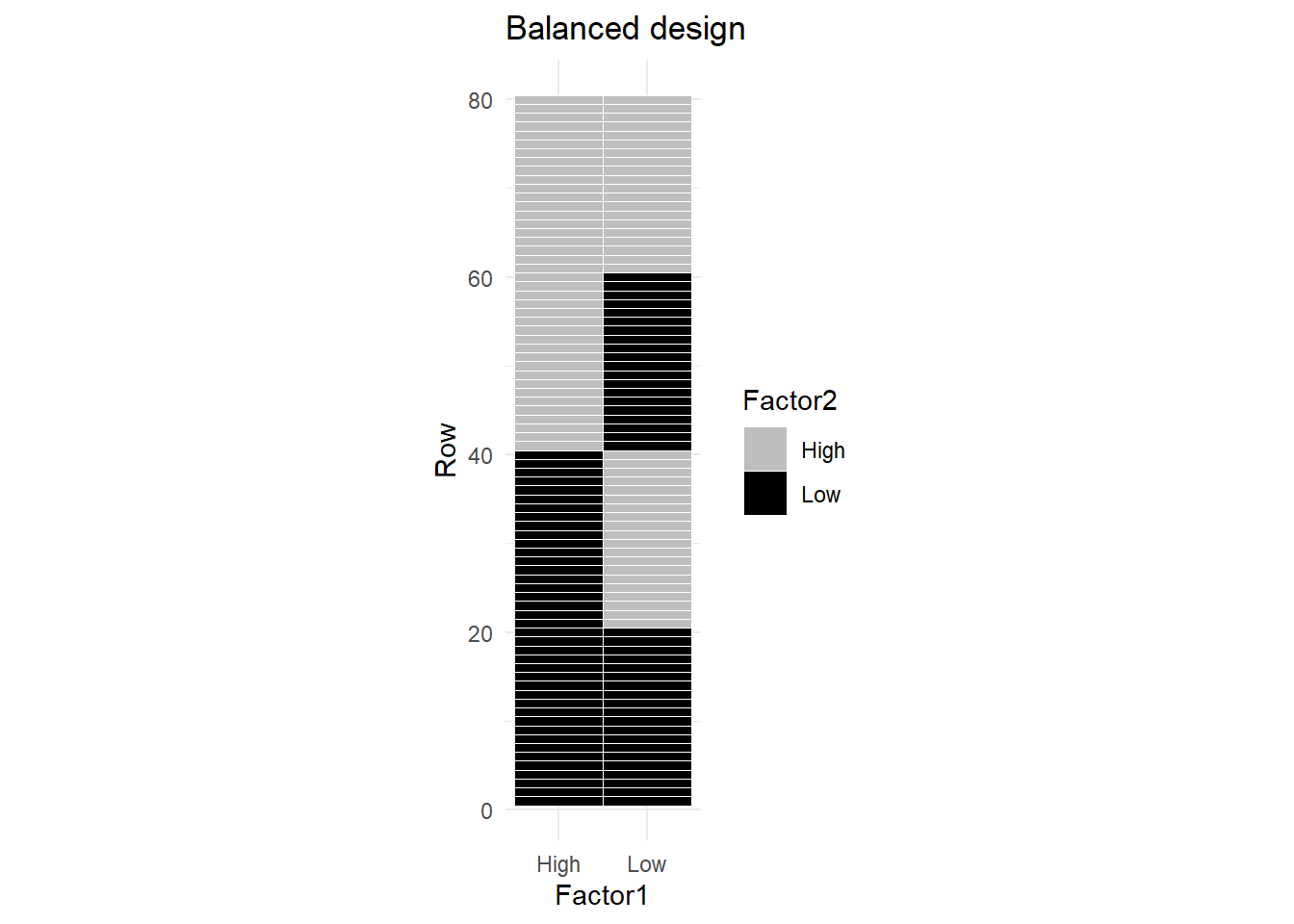
A balanced dataset is one in which there are an equal number of replicates for each and every factor level combination. Unbalanced datasets are those that have an unequal number of replicates in at least one factor level combination and are quite common. In observational studies especially it is more common to have unbalanced data than balanced data. Therefore, it is critical to learn how to analyze unbalanced data.
Though the general principle behind calculating effect sizes still apply (i.e. factor level mean minus sum of all outside factor effects), the effects must be weighted by sample sizes. The formulas for unbalanced data are therefore more complicated than when the data is balanced. This is not an issue since we will let computers do the calculations. The bigger issue deals with the fact that unbalanced datasets often result in correlated factor effects. Due to the equal number of replicates, factors in a balanced dataset are orthogonal. Factors in an unbalanced dataset are not guaranteed this desirable property.1
Figure 1 is a graphical depiction of an unbalanced dataset for two factors, each with 2 levels: High and Low. You can see that each factor level combination appears an equal number of times2.
The correlation of these two factors is zero.
We are measuring the correlation of the coded factors with each other. We have not bothered to define the response variable in these examples, since it is irrelevant to the discussion.
Now consider Figure 2, where there are fewer observations for the combination (Low, Low), and more observations for (Low, High) combination.
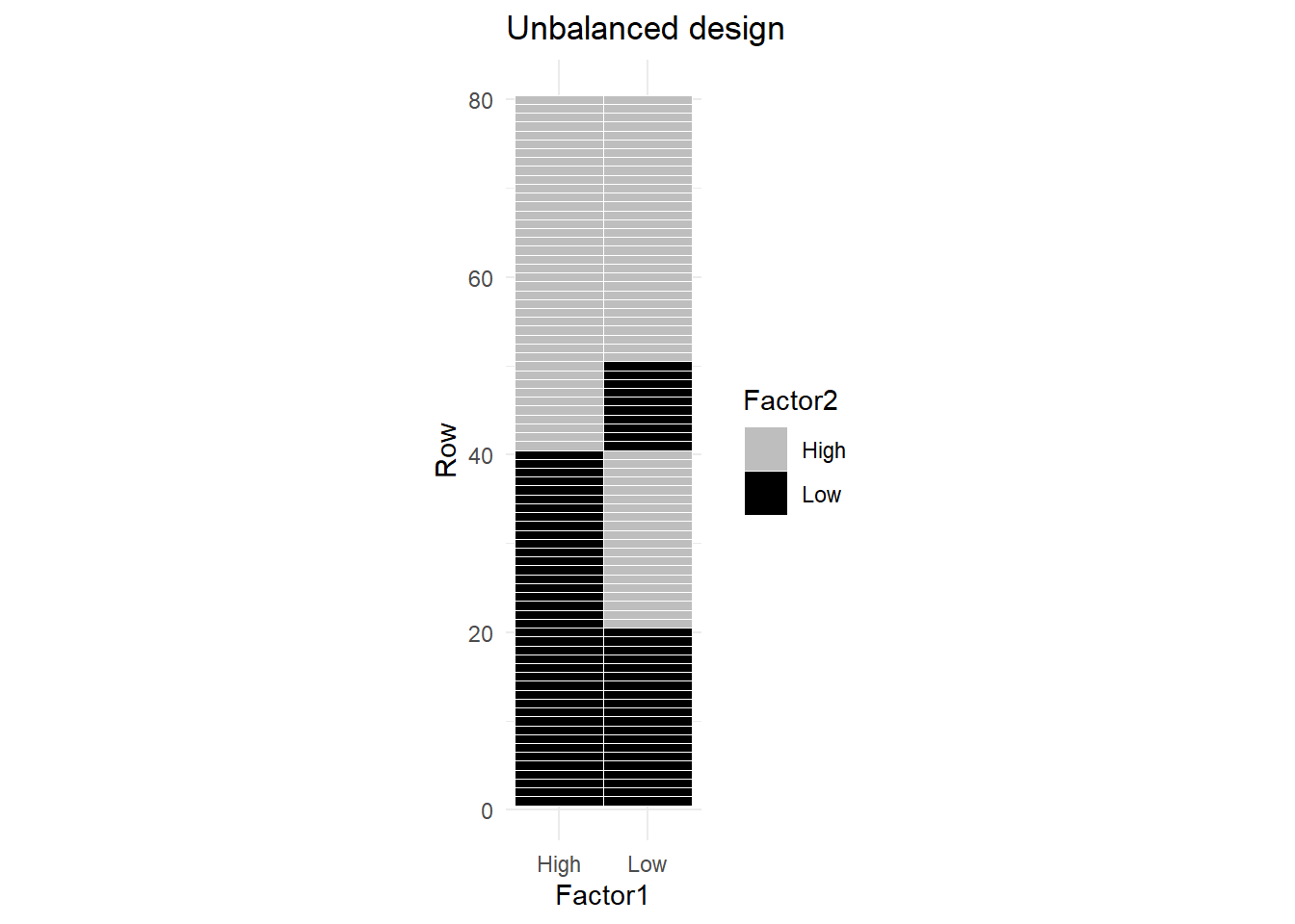
The correlation between the two factors is NOT zero.
The issue with correlated factors is that their effects on the response are also confounded. When the response varies it cannot be determined how much of the variation in the response is due to factor A and how much was due to factor B.
This correlation/confounding of effects also means it is not clear exactly which factor the sums of squares should be attributed to in an ANOVA. Figure 3 (a)3 illustrates this shared sum of squares. The shared sum of squares is due to the correlation between the two factors and is represented by the overlap in the circles.

Warning
The venn diagram in Figure 3 only represents a situation with 2 structural factors, it does NOT include the interaction. An interaction factor would be represented with a third circle, the interaction is not the intersection/overlapping section of A and B factors.
Type I
Sequential Sum of Squares, or Type I, means the order in which terms are specified in the model determines which factor the shared sum of squares is attributed to. This is the default approach in R.
Figure 3 (b) and (c) illustrate how the sum of squares are allocated according to order the factors are listed when the model is specified.
This can be illustrated with a more concrete example, using data to show how sequential sums of squares works. The data are taken from a hypothetical example by Shaw & Mitchell-Olds(1993)4 as cited by Hector, Von Felton, & Schmid (2010)5. In this study, the response is height of a plant. One factor is thinning: yes or no. Thinning is a process where neighboring plants are removed so that they do not compete with each other for light and nutrients in the soil. The other factor in the study is the initial size of the plant at the beginning of the study period. It also has two levels: small and large.
Initial size and thinning were crossed to create an unbalanced BF[2] design. The data are presented in Table 1
Code
example = tibble( initial_size = c(rep("small",5), rep("large", 6)),
        thinning = c("not thinned", "not thinned", rep("thinned", 3), rep("not thinned", 4), "thinned", "thinned"),
        height = c(50, 57, 57, 71, 85, 91, 94, 102, 110, 105, 120))
pander(example)| initial_size | thinning | height |
|---|---|---|
| small | not thinned | 50 |
| small | not thinned | 57 |
| small | thinned | 57 |
| small | thinned | 71 |
| small | thinned | 85 |
| large | not thinned | 91 |
| large | not thinned | 94 |
| large | not thinned | 102 |
| large | not thinned | 110 |
| large | thinned | 105 |
| large | thinned | 120 |
Table 2, below, contains output for the ANOVA when initial_size is listed first in the code where the model is defined. initial_size is highly significant (p-value = .0004) due to the high value for Sum of Squares. thinning is also marginally significant (p-value = 0.0510).
Code
A_first <- aov(height~initial_size + thinning + initial_size:thinning, data = example)
pander(anova(A_first), round = c(0,0,0,2,3))| Df | Sum Sq | Mean Sq | F value | Pr(>F) | |
|---|---|---|---|---|---|
| initial_size | 1 | 4291 | 4291 | 40.17 | 0 |
| thinning | 1 | 590 | 590 | 5.52 | 0.051 |
| initial_size:thinning | 1 | 11 | 11 | 0.11 | 0.753 |
| Residuals | 7 | 748 | 107 | NA | NA |
In Table 2, the \(SS_\text{initial size}\) represents the sum of squares for initial size as if it was the only term in the model. \(SS_\text{thinning}\) is calculated after accounting for all the sum of squares due to initial size. Similarly, the sum of squares for the interaction represents the left over sum of squares that can be attributed to the interaction factor after accounting for initial size and thinning. Thus, each factor represents the remaining sum of squares attributable to that factor after accounting for everything that appeared before it in the model, and ignoring everything that came after it in the model specification.
Observe the changes in Table 3 when we reverse the order of initial_size and thinning in the model specification. thinning is far from significant and has a much lower sum of squares. Thus, the order in which factors are entered into the model is critical.
Don’t worry that \(SS_{thinning}\) was actually lower when thinning was listed first. This sometimes occurs.
Code
thinning_first <- aov(height~thinning + initial_size + thinning:initial_size, data = example)
pander(anova(thinning_first), round = c(0,0,0,2,3))| Df | Sum Sq | Mean Sq | F value | Pr(>F) | |
|---|---|---|---|---|---|
| thinning | 1 | 35 | 35 | 0.33 | 0.583 |
| initial_size | 1 | 4846 | 4846 | 45.37 | 0 |
| thinning:initial_size | 1 | 11 | 11 | 0.11 | 0.753 |
| Residuals | 7 | 748 | 107 | NA | NA |
When specifying the interaction term in R thinning:initial_size is equivalent to initial_size:thinning.
There are a few interesting thing to note when comparing the output in Table 2 with Table 3.
- Even though the sum of squares for the two main effects changed, their total is the same.
\[ 4291 + 590 = 35 + 4846 = 4881 \]
This illustrates a key point about Type I SS: the sum of SS of all the factors will equal \(SS_{total}\).
- The interaction term was the last specified factor in both cases, and so its sum of squares is the same in both tables.
- The \(SS_{residuals}\) does not change based on the order.
Deciding which factor to list first is not always easy and depends on your desired hypotheses. In this case, we may wish to test the effectiveness of thinning after accounting for the effect of the initial size of the plant. If such was the case, it would make sense to list thinning second.
In most basic factorial designs it is not appropriate or possible to decide which variable should be listed first. You can use an adjusted sum of squares approach instead, which include Type II and Type III. We will discuss Type III first since it is more straightforward to explain.
Type III
When sequential sum of squares is not appropriate, one common method of adjustment is called Type III, or “as if last”, sum of squares. This approach computes the sums of squares for each factor as if it was the last factor listed in the sequential sum of squares. To illustrate this, 3 ANOVA tables are shown below. In each table, a different factor is listed last. When the interaction is listed last, it’s sums of squares is 11; when initial_size is listed last its sum of squares is 4,808; and when thinning is listed last its sum of squares is 597 (all values have been rounded to the nearest whole number).
| Df | Sum Sq | Mean Sq | F value | Pr(>F) | |
|---|---|---|---|---|---|
| thinning | 1 | 35 | 35 | 0.3 | 0.58 |
| initial_size | 1 | 4846 | 4846 | 45.4 | 0 |
| interaction | 1 | 11 | 11 | 0.1 | 0.75 |
| Residuals | 7 | 748 | 107 | NA | NA |
| Df | Sum Sq | Mean Sq | F value | Pr(>F) | |
|---|---|---|---|---|---|
| thinning | 1 | 35 | 35 | 0.3 | 0.58 |
| interaction | 1 | 50 | 50 | 0.5 | 0.52 |
| initial_size | 1 | 4808 | 4808 | 45 | 0 |
| Residuals | 7 | 748 | 107 | NA | NA |
| Df | Sum Sq | Mean Sq | F value | Pr(>F) | |
|---|---|---|---|---|---|
| interaction | 1 | 44 | 44 | 0.4 | 0.54 |
| initial_size | 1 | 4252 | 4252 | 39.8 | 0 |
| thinning | 1 | 597 | 597 | 5.6 | 0.05 |
| Residuals | 7 | 748 | 107 | NA | NA |
The type III ANOVA output, in Table 5, contains the sum of squares for each factor when it was listed last.
The order of the variables when coding the model does not matter in a Type 3 ANOVA.
Code
#It doesn't matter which of the 3 models from above that I use since order does not matter when using Type III ANOVA. I will use the model with the interaction as last.

pander(car::Anova(int_last, type = 3,
contrasts = list(thinning = contr.sum, initial_size = contr.sum, interaction = contr.sum)), round = c(0,0,1,2))| Sum Sq | Df | F value | Pr(>F) | |
|---|---|---|---|---|
| (Intercept) | 39402 | 1 | 368.9 | 0 |
| thinning | 597 | 1 | 5.6 | 0.05 |
| initial_size | 4808 | 1 | 45 | 0 |
| interaction | 11 | 1 | 0.1 | 0.75 |
| Residuals | 748 | 7 | NA | NA |
The sum of squares contained in a Type III ANOVA table can be interpreted as the sum of squares attributable to a factor after all the other factors in the model have been accounted for. Type III does not attribute the overlapping sum of squares to any factor. This is represented by the middle intersection piece of the Venn diagram in panel (d) of Figure 3.6 This is why the sum of squares for factors in Type III do NOT add up to the total sum of squares, like they did in Type I.
The Type III ANOVA tests are based on marginal means unweighted by sample size.
Type II
One of the major complaints against a Type III approach is that it violates the principle of marginality. The marginality principle states when a higher order effect (e.g. an interaction) is included in a model, the lower order effects (e.g. main effects) should also be included in the model. According to this principle it does not make sense to test a main effect “as if last” after accounting for the interaction, which is exactly the situation we came across in Type III (see Table 5, panel b and c).
Type II strives to maintain the principle of marginality, while at the same time taking an “as if last” approach. Stated another way, in a Type II ANOVA, each factor is tested “as if last” but ignoring all terms that contain that factor.
To illustrate this, 2 different Type I ANOVA tables are shown in Table 6. (Note: These are actually the same tables presented in explanation of Type I). In each table, the order of the main effects is swapped, while the higher order interaction always appears afterward.
| Df | Sum Sq | Mean Sq | F value | Pr(>F) | |
|---|---|---|---|---|---|
| thinning | 1 | 35 | 35 | 0.3 | 0.58 |
| initial_size | 1 | 4846 | 4846 | 45.4 | 0 |
| thinning:initial_size | 1 | 11 | 11 | 0.1 | 0.75 |
| Residuals | 7 | 748 | 107 | NA | NA |
| Df | Sum Sq | Mean Sq | F value | Pr(>F) | |
|---|---|---|---|---|---|
| initial_size | 1 | 4291 | 4291 | 40.2 | 0 |
| thinning | 1 | 590 | 590 | 5.5 | 0.05 |
| initial_size:thinning | 1 | 11 | 11 | 0.1 | 0.75 |
| Residuals | 7 | 748 | 107 | NA | NA |
The type II ANOVA output, in Table 7, contains the sum of squares from Table 6. Specifically, the Sum of Squares in Table 7 for thinning is 590 because that is the Sum of Squares in Table 6 panel b, when “thinning” was the last main effect listed. Similarly, the Sum of Squares in Table 7 for initial_size is 4846 because that is the Sum of Squares from Table 6 panel a, when “initial_size” was the last main effect listed.
| Sum Sq | Df | F value | Pr(>F) | |
|---|---|---|---|---|
| thinning | 590 | 1 | 5.5 | 0.05 |
| initial_size | 4846 | 1 | 45.4 | 0 |
| thinning:initial_size | 11 | 1 | 0.1 | 0.75 |
| Residuals | 748 | 7 | NA | NA |
The sum of squares contained in a Type II ANOVA table can be interpreted as the sum of squares attributable to a factor after all other factors that it is not a part of in the model have been accounted for.
A succinct and general explanation from a website is pasted below:
The Type II ANOVA tests are based on marginal means weighted by sample size.
Specifically, for a two-factor structure with interaction, the main effects A and B are not adjusted for the AB interaction because the interaction contains both A and B. Factor A is adjusted for B because the symbol B does not contain A. Similarly, B is adjusted for A. Finally, the AB interaction is adjusted for each of the two main effects because neither main effect contains both A and B. Put another way, the Type II SS are adjusted for all factors that do not contain the complete set of letters in the effect. …[It allows] lower-order terms explain as much variation as possible, adjusting for one another, before letting higher-order terms take a crack at it.
Consider a 3-way model, with factors A, B, and C. The Type II sums of squares for factor A are calculated as SS(A | B, C, BC). In other words, A’s contribution to the variance is calculated after accounting for the contribution of factors B, C, and B*C. The sum of squares for factor AB are calculated as SS(AB | A, B, C, AC, BC).
Other Sum of Squares Types
There are actually many other methods for calculating sum of squares, and they have been given type numbers as well. However, these other types are rarely used. They are often very complex and don’t have clear interpretations. They also may be dependent on how the factors are coded (which level is a reference category for example).
Pros/Cons Table
Below is a summary table of the pros and cons of the first 3 methods.
| ANOVA Type | Pros | Cons |
|---|---|---|
| Type I |
|
|
| Type II |
|
|
| Type III |
|
|
After decades of debate and disagreement, there is an emerging concept gaining ground among statisticians that there doesn’t have to be a “right” and a “wrong” approach. Rather, the analyst should pick the approach that best matches the hypothesis they wish to test.
More Guidance on When to Use Which Type
Knowing which type to use is difficult, but can be summarized with a simple decision tree.7
Do you have strong theoretical consideration to inflate the importance of one of your variables?
- If Yes, use Type I. (Place the variable with the greatest importance first)
- If No, proceed to question 2.
Is an interaction expected between the independent factors?
- If Yes, use Type III
- If No, use Type II
Examples
This section strives to provide an example of when each type of ANOVA may be appropriate.
Type I
For an example of when Type I may be useful we do not need to look any further than the plant study we have been using all along on this page. Say our research question aims to test the effectiveness of thinning after accounting for the plant’s initial size our hypothesis matches a Type I approach. The research question specifies the order in which we want to consider the factors. Since Type I ANOVA is dependent on the order in which factors are specified in the model, we are able to incorporate the desired order from our research question into the analysis.
Type II
You may want to use a Type II ANOVA if the disparity in sample sizes reflects a similar disparity in population size. Perhaps your end goal is to apply the treatment to all members of the population and you want any difference observed in the study to be present in the population. In that case, Type II may be the best choice. This will be more common in observational studies.
For example, a web developer randomly assigns website visitors to one of two website designs. The population that visits this website is predominantly male. Therefore, Design A and Design B receive many more males than females. In this case, the lopsided nature of the gender distribution may accurately reflect the population of website visitors being predominantly male.
Notice that this example’s decision is motivated by an explanation of weighted vs. non-weighted means. However, the decision tree still applies. In this Type 2 example, the interaction effect of gender by website is essentially ignored (or saved for last), letting the main effects try to explain as much of the variation as possible without controlling for the imbalance in factor level combinations.
The test of the main effects for gender and website design will be influenced by sample sizes. Say we conclude that people tend to buy more products when presented with website B. This conclusion will be influenced more heavily by males since males represented a larger proportion of the sample. But in this case that’s okay because males also represent a larger part of our target audience (website visitors).
Type III
Let’s continue with the website design and gender study mentioned above. Now, instead of taking the role of a business owner, we assume the role of a cognitive psychologist. We are not interested in trying to maximize profits for a target market. Rather, we are interested in knowing how individuals respond to the two different site designs. The fact that we partnered with a website with predominantly male clientele is incidental. We want to arrive at conclusions that will be useful in explaining/predicting behavior of an individual.
If we use Type II ANOVA the result of the significance test of website design will not account for the fact that males account for a larger portion of the sample. A Type III ANOVA will not weight by sample size and will treat the estimated means of males and females equally. Thus our results can be used to predict an individual’s behavior based on their gender and website design. Our findings can now be used by other websites with a different clientele (e.g. predominantly female) to correctly predict/explain individual’s actions.
Key Points
A few other key points are worth remembering.
First, small amount of unbalance will result in a small amount of difference in the different methods for calculating sum of squares. When the data is balanced, the 3 types of ANOVA will give the same results.
Second, no amount of adjustment to the sum of squares calculation can account for or correct bias in a study. For this reason, it is important to understand what is causing the unbalance in the dataset. Was it a deliberate decision in the design due to time/cost constraints? Was it due to spoiled experimental runs/units? In the case of human research, was attrition the cause? If the cause of the unbalance is related to the factor level values there could be bias in the study.
For example, consider an experiment that wanted to study people’s sentiment about public speaking. One group of 10 participants was assigned to talk about their most embarrassing moment. The other group of 10 participants was assigned a neutral topic, like what they had for dinner the previous day. Four of the 10 people assigned to speak on an embarrassing moment dropped out of the study. The design started out as balanced, but the resulting dataset is unbalanced.
The reason for multiple people dropping out is likely connected to the fact that those people may not feel comfortable sharing embarrassing experiences in a public setting. The remaining people in the study may be fundamentally different in how they feel about sharing embarrassing experiences. The data is not missing completely at random. Bias has been introduced!
Third, always test your highest-order interaction first. The results for the highest order interaction will be the same regardless of what type of ANOVA you use (sequential or adjusted). If the interaction is significant, most of the time it is not appropriate to interpret the hypothesis test of the main effects anyway so you won’t need to worry about which type is used.
Finally, when analyzing unbalanced data in this class you should use Type III ANOVA unless directed otherwise. This ends up being a bit of a conservative approach. If a main effect is significant, even after accounting for a non-significant interaction, there is a good chance the main effect will be even more significant if the interaction were to be excluded. The Type III is also simpler in terms of explanation/interpretation. It will help share answers and work if we are all using the same approach as a class.
Tip
Use Type III ANOVA for unbalanced datasets in this class.
R Instruction
Type I ANOVA is the default in the anova() command. In fact, it is the only type of ANOVA available in anova().
To get Type II or Type III ANOVA you will create a model in the usual way and and redefine the way the model is parameterized using a contrasts8 argument. Then use the Anova() command from the car package. Note the use of the capital ‘A’, instead of lower case ‘a’, in the function name.
myaov <- aov(y ~ factorA * factorB,
             contrasts = list(factorA = contr.sum, factorB = contr.sum), data = df)
car::Anova(myaov, type = 3)myaovis the name we give our model in the first line of code.contrastsargument tells R how to parameterize the X matrix. In other words, R actually changes a factor variable into a series of columns to represent the various levels. This tells R what values should go in those columns. The default values for contrasts will result in garbage results when used with theAnova()command.caris the name of the package theAnova()command comes from::allows you to use functions from a package without having to load the entire package with alibrary()command. The package you want to access is specifed on the left of the::and the function name is specified on the right.Anova()is a function from thecarpackage. It can be used to get type II or type III ANOVA tables for a variety of different models, includingaov(),lm(),glm(), etc.type=argument specifies whether Type II or Type III is desired. It accepts Arabic numerals, or roman numerals in quotes: 2, 3, “II”, “III”. The default, if this argument is omitted, is Type 2.
Alternative Code
Rather than adding a contrasts argument to each of your aov() statements, you can set the contrasts in the options once. Then all subsequent models will use those types of contrasts. Run this code:
options(contrasts = c("contr.sum", "contr.poly"))
or
options(contrasts = c("contr.sum", "contr.sum"))
Notice there are two values needed in the contrasts input vector. The first specifies how to handle unordered categorical variables, the second specifies how to handle ordered categorical variables. The default contrasts in R (in case you need to revert back) is options(contrasts = c("contr.treatment", "contr.poly")).
summary()
Many students are in the habit of using summary() to evaluate model hypothesis tests. When called on an aov object (i.e. an object created using the aov() command), summary()’ prints a Type I ANOVA table.
However, when called on an lm() object, summary() does not print an ANOVA table at all. The default output is to print variable coefficients, standard deviations, and t-test results (t statistic and p-value). If the object has an independent, categorical factor variable a t-test will be conducted for the factor levels. (Actually, all but 1 factor level will be tested. The missing factor level is considered the reference level and is included in the intercept. The reference level is whatever level comes first alphabetically, unless defined otherwise.). If there are only two factor levels, the p-value from the t-test of that factor will be equal to the p-values from a Type III ANOVA applied to the same model.
To get an ANOVA table and the F-tests for a factor’s overall significance you can call car::Anova() or anova() on an lm() object.
Footnotes
For a brief, accessible description of how orthogonality relates to balanced designs, read here: https://www.statisticshowto.com/orthogonality/. The last sentence states “Orthogonality is present in a model if any factor’s effects sum to zero across the effects of any other factors in the table.” We know a factor’s effects sum to zero, and when factors are crossed, the above quoted statement is also true IF there are an equal number of replicates at each factor level. When the number of replicates is not equal, the sum across factor levels is not guaranteed to be exactly zero; so, orthogonality is no longer guaranteed.↩︎
https://stats.stackexchange.com/questions/552702/multifactor-anova-what-is-the-connection-between-sample-size-and-orthogonality↩︎
Journal of Animal Ecology, Volume: 79, Issue: 2, Pages: 308-316, First published: 05 February 2010, DOI: (10.1111/j.1365-2656.2009.01634.x)↩︎
Shaw, R.G. & Mitchell-Olds, T. (1993) ANOVA for unbalanced data: an overview. Ecology, 74, 1638–1645.↩︎
Journal of Animal Ecology, Volume: 79, Issue: 2, Pages: 308-316, First published: 05 February 2010, DOI: (10.1111/j.1365-2656.2009.01634.x)↩︎
There is also the possibility the total sum of squares is more than the sum of squares total due to “double counting” the variation. This is much more difficult to illustrate with Venn diagrams.↩︎
This discussion has assumed the model is using fixed effects for all factors. In random effects models or mixed models the discussion changes. Those models are outside the scope of this book.↩︎
In R, when you’re fitting a linear model using the
lm()oraov()function, thecontrastsargument allows you to specify how categorical variables should be encoded into dummy variables for regression analysis.By default, R uses treatment contrasts, where one level of the categorical variable is chosen as the reference level, and the coefficients for the other levels are compared to this reference level. However, you can change this behavior using the
contrastsargument to specify different types of contrasts, such as “contr.sum”, “contr.poly”, “contr.helmert”, etc., each of which results in a different encoding of the categorical variables.For example, if you have a categorical variable “gender” with levels “male” and “female” and you want to use sum contrasts where the coefficients represent the sum of the response variable for each level compared to the overall mean [which is how we have defined effects in this class], you would specify
contrasts = list(gender = contr.sum)in theaov()function.Here’s a brief overview of some common contrast options:
- Contr.sum: Contrasts sum to zero. Useful for testing specific hypotheses, as it directly compares each group to the overall mean.
- Contr.treatment: Default behavior in R. One level is chosen as the reference, and the coefficients represent differences from this reference level.
- Contr.poly: Polynomial contrasts. Useful for ordinal categorical variables where you want to model linear, quadratic, cubic, etc., trends.
- Contr.helmert: Helmert contrasts. Each level is compared to the mean of subsequent levels.
- Contr.SAS: Similar to Helmert contrasts, but with a different ordering of coefficients.
These are just a few examples; there are more contrast options available in R. The choice of contrast depends on the specific research question and the nature of the categorical variable.
From a ChatGPT 3.5 conversation in May, 2024.↩︎