This section will extend a factorial design with two factors to a full factorial design with three factors. The design and analysis of a fully factorial experiment with three factors is very similar to the two factor design. The one notable exception is that now there is the potential for higher order interactions. Instead of just a single two-way interaction to be considered, three-way interactions, as well as all possible two-way interactions, are included in the model
To illustrate this design and analysis we will use a fictitious dataset that closely mirrors the real experiment conducted by Robert Kaplan. The experiment’s goal was to show how the halo effect due to attractiveness effects influences an assessment. More precisely, how does an author’s attractiveness, their sex, and the sex of the reader impact the reader’s assessment of the author’s talent as a writer.
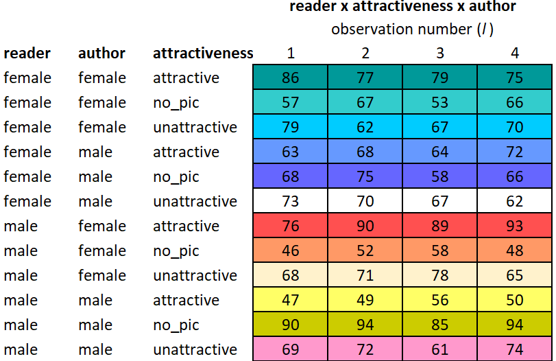
To carry out the experiment, a participant is treated as the reader. There were 48 readers total, 24 male and 24 female. The participant is asked to read an essay. Though all participants read the same essay, the sex of the author and the attractiveness of the author was varied. This was accomplished by attaching a picture of the author to the essay. There were 3 levels of attractiveness for each author sex: attractive, unattractive, and the control group (where no picture was attached). Each reader was randomly assigned to an author sex and attractiveness level such that for every combination of reader sex, author sex, and author attractiveness there were exactly 4 observations gathered, resulting in a total of 48 observations.
It is cleaner and easier to show the data in a different format than has been used up to this point. In Table 1, each factor has a column dedicated to show what factor level the observations in that row belong to. There are 12 unique factor level combinations, and therefore 12 rows in the table There are 4 observations per factor level combination, and they are displayed to the right of factor level combination designation.
Table 1: Table of Means for Each Factor Level Combination
row
reader
author
attractiveness
1
2
3
4
1
female
female
attractive
47
49
56
50
2
female
female
no-pic
69
72
61
74
3
female
female
unattractive
90
94
85
94
4
female
male
attractive
63
68
64
72
5
female
male
no-pic
73
70
67
62
6
female
male
unattractive
68
75
58
66
7
male
female
attractive
76
90
89
93
8
male
female
no-pic
68
71
78
65
9
male
female
unattractive
46
52
58
48
10
male
male
attractive
86
77
79
75
11
male
male
no-pic
79
62
67
70
12
male
male
unattractive
57
67
53
66
Factor Structure
We can still partition the observations, but with 3 factors the partitions become harder to show with just lines. Instead, the partitions will be described and a table of factor levels will be shown below.
In the appendix, partitioning is done using shading/coloring of cells. Though it is possible, the result is a bit overwhelming to the eye.
In this experiment there are 3 controlled factors. Observations can be partitioned according to what group they belong to for any one of the 3 controlled factors. This allows us to create 3 structural factors, 1 for each controlled factor:
reader’s sex: 2 levels.
author’s sex: 2 levels, and
attractiveness (of the essay author): 3 levels,
The partition associated with each of these factors will allow us to calculate main effects.
The data can also be partitioned according to a shared factor level combination on a pair of factors. There are 3 possible factor pairs. In other words, three two-way interactions are created by partitioning the data this way:
Finally, data values can be partitioned according to what combination of the 3 treatment factors the observation belongs to. This results in a 3-way interaction factor:
\(y_{ijkl}\) is the \(l^{th}\) observation from the factor level combination of \(\alpha_i\), \(\beta_j\), and \(\gamma_k\).
\(\mu\) is the grand mean of all the observations.
\(\alpha\) is the effect of reader’s gender, and \(i\) has 2 levels: i=1 for female, i=2 for male
\(\beta\) is the effect of author’s gender, and \(j\) has 2 levels: i=1 for female, i=2 for male
\(\gamma\) is the effect of author’s attractiveness, and \(k\) has 3 levels: k=1 for attractive, k=2 for neutral, and k=3 for unattractive
The \((\alpha\beta)_\text{ij}\) is the interaction effect for reader gender with author gender on perceived talent level.
The \((\alpha\gamma)_\text{ik}\) is the interaction effect for reader gender with author attractiveness on perceived talent.
The \((\beta\gamma)_\text{jk}\) is the interaction effect for author gender with attractiveness on perceived talent.
The \((\alpha\beta\gamma)_\text{ijk}\) is the interaction effect for reader gender, author gender, and attractiveness on perceived talent.
\(\epsilon\) is the residual error term, and \(l\) is the replicate count within a factor level combination.
Though we have seen two factor interactions and know how to deal with them, the three factor interaction is something new. Including this term in the model means that the impact of any of the three variables depends on the levels of the other two. Stated another way, the nature of the two-way interaction depends on the level of a third variable.
The main effects and two-way interactions are tested just as they were in the BF[2] model. The hypothesis for the 3-way interaction is
\[
H_0: (\alpha\beta\gamma)_\text{ijk} = 0 \text{ for all } ijk
\]
\[
H_a: (\alpha\beta\gamma)_\text{ijk} \ne 0 \text{ for some } ijk
\]
Assumptions
A three-way ANOVA model may be used to analyze data from a BF[3] design if the following requirements are satisfied. Note that these requirements are identical to the requirements of a BF[2] two-way ANOVA.
Requirements
Method for Checking
What You Hope to See
Constant variance across factor levels
Residual vs. Fitted Plot
No major disparity in vertical spread of point groupings
Levene’s Test
Fail to reject \(H_0\)
Normally Distributed Residuals
Normal Q-Q plot
Straight line, majority of points in boundaries
Independent residuals
Order plot
No pattern/trend
Familiarity with/critical thinking about the experiment
No potential source for bias
Design
In a basic factorial design of 3 factors, three factors are purposely varied in such a way that observations are obtained for every possible factor level combination. Each factor level combination is considered a treatment.
In a completely randomized design, each experimental unit is randomly assigned to exactly 1 factor level combination. It can be helpful to first list out all the subjects and factor level combinations in a table. This can be done by listing all the subjects, then listing the values of each factor in a separate column.
There are 12 unique factor level combinations. If we want to observe each factor level combination 4 times, we need \(12 \times 4 = 48\) observations.
#Create a sequence from 1 to 48#Paste the word "Subject " in front of each id #Subject <-paste("Subject", seq(1:48), sep =" ")#Create a vector with each reader gender repeated 24 timesreader <-rep(c("female", "male"), each =24)#Create a vector with each author gender repeated 24 timesauthor <-rep(c("female", "male"), each =12, times =2)#Create a vector with each level of attractiveness repeated 16attractiveness <-rep(c("attractive", "neutral", "unattractive"), times =16)#Combine the vectors of Subject ID's and controlled factor levels into one tibble/datasetassignment_table <-tibble(Subject, reader, author, attractiveness)#print the table, pander() makes it look nicepander(assignment_table)
Subject
reader
author
attractiveness
Subject 1
female
female
attractive
Subject 2
female
female
neutral
Subject 3
female
female
unattractive
Subject 4
female
female
attractive
Subject 5
female
female
neutral
Subject 6
female
female
unattractive
Subject 7
female
female
attractive
Subject 8
female
female
neutral
Subject 9
female
female
unattractive
Subject 10
female
female
attractive
Subject 11
female
female
neutral
Subject 12
female
female
unattractive
Subject 13
female
male
attractive
Subject 14
female
male
neutral
Subject 15
female
male
unattractive
Subject 16
female
male
attractive
Subject 17
female
male
neutral
Subject 18
female
male
unattractive
Subject 19
female
male
attractive
Subject 20
female
male
neutral
Subject 21
female
male
unattractive
Subject 22
female
male
attractive
Subject 23
female
male
neutral
Subject 24
female
male
unattractive
Subject 25
male
female
attractive
Subject 26
male
female
neutral
Subject 27
male
female
unattractive
Subject 28
male
female
attractive
Subject 29
male
female
neutral
Subject 30
male
female
unattractive
Subject 31
male
female
attractive
Subject 32
male
female
neutral
Subject 33
male
female
unattractive
Subject 34
male
female
attractive
Subject 35
male
female
neutral
Subject 36
male
female
unattractive
Subject 37
male
male
attractive
Subject 38
male
male
neutral
Subject 39
male
male
unattractive
Subject 40
male
male
attractive
Subject 41
male
male
neutral
Subject 42
male
male
unattractive
Subject 43
male
male
attractive
Subject 44
male
male
neutral
Subject 45
male
male
unattractive
Subject 46
male
male
attractive
Subject 47
male
male
neutral
Subject 48
male
male
unattractive
Now randomize which subjects get which treatment (aka - factor level combination).
#randomize subject assignment to treatmentrandomized_table <-tibble(sample(Subject), reader, author, attractiveness)#print the table, pander() makes it look nicepander(randomized_table)
sample(Subject)
reader
author
attractiveness
Subject 28
female
female
attractive
Subject 25
female
female
neutral
Subject 33
female
female
unattractive
Subject 24
female
female
attractive
Subject 19
female
female
neutral
Subject 40
female
female
unattractive
Subject 20
female
female
attractive
Subject 21
female
female
neutral
Subject 37
female
female
unattractive
Subject 29
female
female
attractive
Subject 35
female
female
neutral
Subject 18
female
female
unattractive
Subject 8
female
male
attractive
Subject 1
female
male
neutral
Subject 48
female
male
unattractive
Subject 13
female
male
attractive
Subject 32
female
male
neutral
Subject 31
female
male
unattractive
Subject 7
female
male
attractive
Subject 23
female
male
neutral
Subject 42
female
male
unattractive
Subject 38
female
male
attractive
Subject 17
female
male
neutral
Subject 6
female
male
unattractive
Subject 26
male
female
attractive
Subject 36
male
female
neutral
Subject 3
male
female
unattractive
Subject 11
male
female
attractive
Subject 30
male
female
neutral
Subject 43
male
female
unattractive
Subject 34
male
female
attractive
Subject 10
male
female
neutral
Subject 5
male
female
unattractive
Subject 4
male
female
attractive
Subject 45
male
female
neutral
Subject 41
male
female
unattractive
Subject 46
male
male
attractive
Subject 12
male
male
neutral
Subject 27
male
male
unattractive
Subject 47
male
male
attractive
Subject 15
male
male
neutral
Subject 22
male
male
unattractive
Subject 44
male
male
attractive
Subject 39
male
male
neutral
Subject 14
male
male
unattractive
Subject 16
male
male
attractive
Subject 2
male
male
neutral
Subject 9
male
male
unattractive
Interaction
We can visually investigate main effects and two-way interactions in the same way that was explained on the BF[2] page. To visually inspect the possibility of a 3-way interaction, you can create two-way interaction charts faceted by the third variable.
A chart to inspect a two-way interaction consists of plotting the mean of each factor level combination
It technically does not matter which of the three variables in the interaction you use for faceting, if a three way interaction is there it should be visible. However, it sometimes can be easier to spot the interaction or be more intuitive to interpret the interaction when faceting on one variable instead of another.
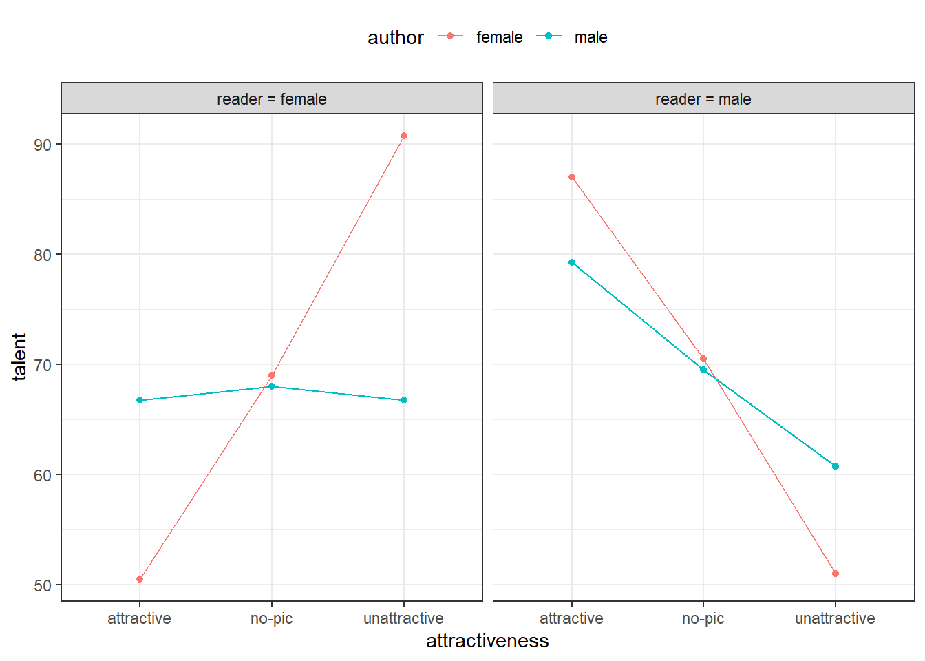
For the study on the halo effect of attractiveness example, we start by computing the mean perceived talent level of our observed data, contained in Table 1. The means are shown in Table 2 and the interaction plots created from those means are shown in Figure 1.
Table 2: Means for Each Factor Level Combination
Group means for Female reader
author
attractive
no-pic
unattractive
female
50.5
69
90.75
male
66.75
68
66.75
Group means for Male reader
author
attractive
no-pic
unattractive
female
87
70.5
51
male
79.25
69.5
60.75
Figure 1: Author Gender and Attractiveness Interaction Plots Faceted by Reader Gender
The plot on the left shows factor levels means when the reader was female. A two-way interaction seems likely based on the way the lines cross. Specifically, female readers rate female authors as more talented when the author is unattractive - kind of a reverse halo effect. However, female readers assessment of male authors does not seem influenced by attractiveness of male authors.
The nature of the interaction between author gender and attractiveness on perceived talent drastically changes when the reader is male, as shown in the plot on the right. Males rate authors of both genders as more talented if the author is more attractive. Thus, this is a good example of a 3 way interaction: the nature of the interaction between author gender and attractiveness depends on the reader’s gender.
Decomposition
In a full factorial design with 3 controlled factors, there are a total of 7 structural factors. Diagramming their partitions can become unwieldy and messy. However, in order to use the general rules to calculate degrees of freedom and factor effects, it is still important to know which factors are inside/outside of other factors.
In a completely randomized, basic factorial experiment, a higher-order interaction is always inside of the factors that make it up. For example, in the halo effect experiment, the interaction between attractiveness and author gender is inside of both attractiveness and author gender. The two-way interactions are neither inside nor outside of each other. For example, reader gender \(\times\) author gender is not inside nor outside of reader gender \(\times\) author attractiveness.
The 3-way interaction of reader gender \(\times\) author gender \(\times\) author attractiveness is inside of the other 6 structural factors (3 main effect factors and 3 two-way interactions).
Factor Effects
The first step in performing a decomposition is to calculate the factor level means. The grand mean is 69.1458333.
The mean for each factor and its corresponding levels is displayed below.
Table 3: Means for Each Factor Level Combination
Mean Talent by Reader Gender
reader
mean
female
68.62
male
69.67
Mean Talent by Author Gender
author
mean
female
69.79
male
68.5
Mean Talent by Author Attractiveness
attractiveness
mean
attractive
70.88
no-pic
69.25
unattractive
67.31
Mean Talent by Reader Gender x Author Gender
reader
author
mean
female
female
70.08
female
male
67.17
male
female
69.5
male
male
69.83
Mean Talent by Reader Gender x Author Attractiveness
reader
attractiveness
mean
female
attractive
58.62
female
no-pic
68.5
female
unattractive
78.75
male
attractive
83.12
male
no-pic
70
male
unattractive
55.88
Mean Talent by Author Gender x Author Attractiveness
author
attractiveness
mean
female
attractive
68.75
female
no-pic
69.75
female
unattractive
70.88
male
attractive
73
male
no-pic
68.75
male
unattractive
63.75
Mean Talent by Reader Gender x Author Gender x Author Attractiveness
reader
author
attractiveness
mean
female
female
attractive
50.5
female
female
no-pic
69
female
female
unattractive
90.75
female
male
attractive
66.75
female
male
no-pic
68
female
male
unattractive
66.75
male
female
attractive
87
male
female
no-pic
70.5
male
female
unattractive
51
male
male
attractive
79.25
male
male
no-pic
69.5
male
male
unattractive
60.75
We will now compute the factor level effects. A couple of example computations for the interaction factors are shown below. The general rule for factor level effects is implemented, it states that the size of an effect is equal to the factor level mean minus the sum of the effects of all outside factors. The computation for each effect of each factor will not be shown.
The full factorial model, as defined in Equation 1, will be used to describe the calculations.
First, let’s compute the effect of a male reader\(\times\) attractive author on perceived talent.
Thus, as we saw earlier in Figure 1, the effect of being attractive is made greater when the reader is a male. Specifically, the mean talent ratings is 11.72 points higher predicted by adding the effect of male reader and the effect of attractive author to the grand mean separately.
To calculate the effect of a three-way interaction, the general rule is again applied. This time though, there are more calculations since all two-way interactions are inside of the 3 way interaction. Below, the effect of male reader\(\times\) female author \(\times\) attractive author is calculated.
Thus, their appears to be a synergistic effect on perceived talent when all three of the levels male reader\(\times\) female author \(\times\) attractive author are present together. Specifically, the mean talent rating is 6.82 points higher than the partial fit (which only includes main effects and two-way interaction effects) would have predicted.
Similar calculations can be done for every factor level effect.
Degrees of Freedom
Degrees of freedom can also be calculated using the general rule: degrees of freedom for a factor is equal to the levels of that factor minus the sum of degrees of freedom for all outside factors. The degrees of freedom calculations are only shown for two factors, leaving it up to the reader to calculate/verify the degrees of freedom for the other factors as presented in the ANOVA summary table in XXX.
The degrees of freedom calculation for the reader by attractiveness interaction factor is shown below. There are 2 reader gender levels \(\times\) 3 attractiveness levels = 6 total levels for this interaction factor.
The three way interaction also has two degrees of freedom.
Completing the ANOVA Table
After degrees of freedom and effects for each factor are calculated, the remaining pieces of the ANOVA table can also be calculated.
To calculate sum of squares for a factor, the effects of each factor level associated with that factor are squared and then multiplied by the number of replicates in that level.1 These products are then summed across levels to get the total sum of squares for the factor.
To obtain the mean squares for a factor, the factor’s sum of squares is divided by the factor’s degrees of freedom.
Finally, the F-statistic is obtained by computing the ratio of a factor’s mean square to the mean squared error. The degrees of freedom associated with this F statistic are the degrees of freedom for the factor and the degrees of freedom for error. The p-value is obtained by finding the area under the F distribution to the right of the F statistic.
Analysis in R
We will illustrate the R code used for a BF[3] analysis halo effect experiment that has been used throughout this page.
Describe the Data
When working with a dataset you should get to know your data through numerical and graphical summaries. Numerical summaries typically consist of means, standard deviations, and sample sizes for each factor level. Graphical summaries most usually are boxplots, scatterplots, and/or interaction plots with the means displayed.
Interactive code and additional explanations of numerical summaries and plots in R are found at R Instructions->Descriptive Summaries section of the book.
So far, we have already seen various numerical and graphical summaries of the data on this page. This summaries below would be a good starting point if you are taking a look at the data for the first time.
Numerical Summaries
A good place to start is calculating summary statistics like mean, standard deviation and sample size for the factor levels of each experimental factor.
Code
#Note: the df data frame was created in the first R chunk in the Overview section of this pagedf %>%group_by(reader) %>%summarise(mean =mean(talent),n =n(),std_dev =sd(talent),.groups ='keep') %>%pander(caption ="Numerical Summary by Reader Gender")df %>%group_by(author) %>%summarise(mean =mean(talent),n =n(),std_dev =sd(talent),.groups ='keep') %>%pander(caption ="Numerical Summary by Author Gender")df %>%group_by(attractiveness) %>%summarise(mean =mean(talent),n =n(),std_dev =sd(talent),.groups ='keep') %>%pander(caption ="Numerical Summary by Attractiveness Gender")
Table 4: Numerical Summaries of Experimental Factors
Numerical Summary by Reader Gender
reader
mean
n
std_dev
female
68.62
24
12.79
male
69.67
24
13.18
Numerical Summary by Author Gender
author
mean
n
std_dev
female
69.79
24
16.67
male
68.5
24
7.684
Numerical Summary by Attractiveness Gender
attractiveness
mean
n
std_dev
attractive
70.88
16
15.02
no-pic
69.25
16
5.31
unattractive
67.31
16
16.04
Much of the above information can also be seen in an effective visual.
Graphical Summaries
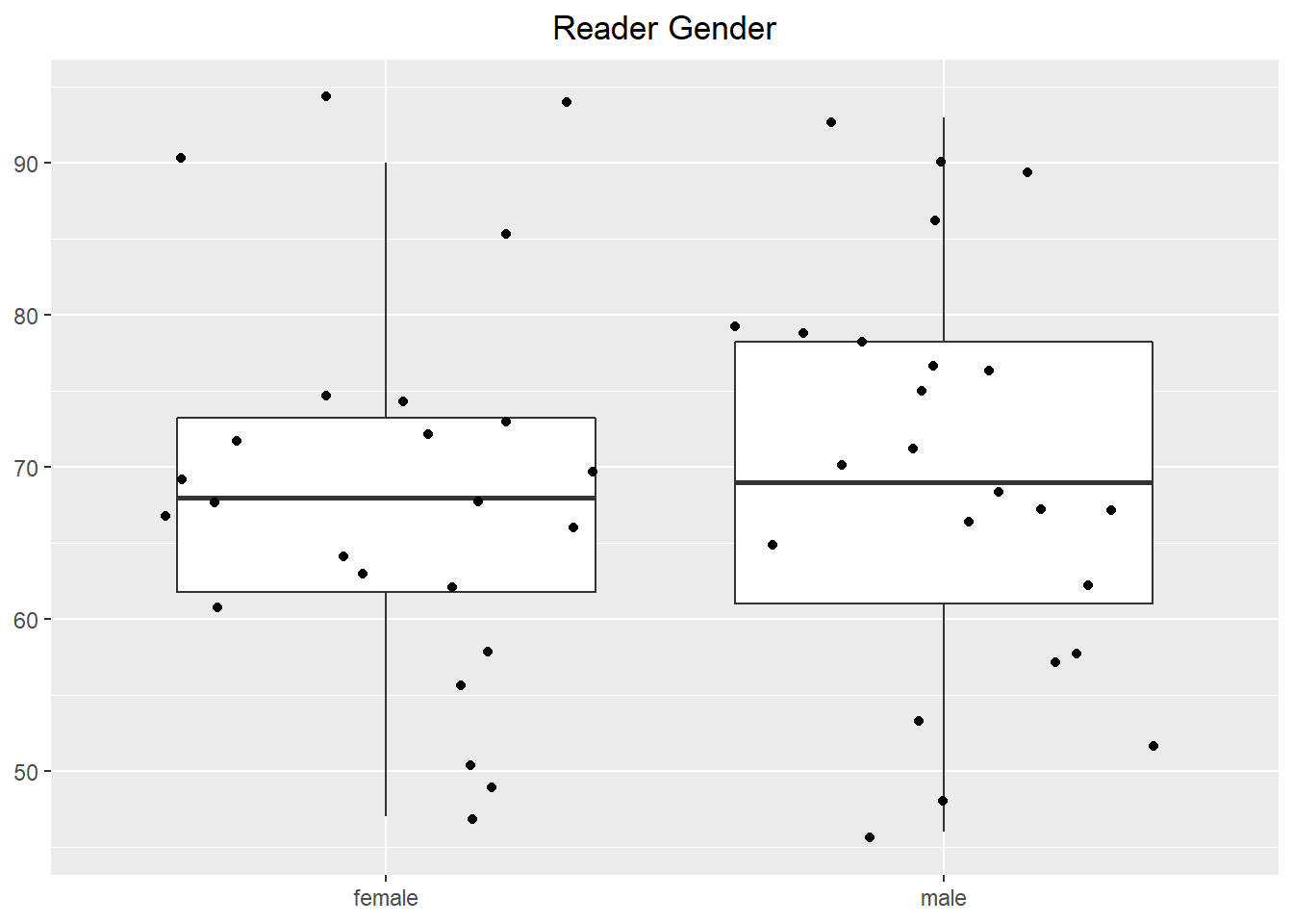
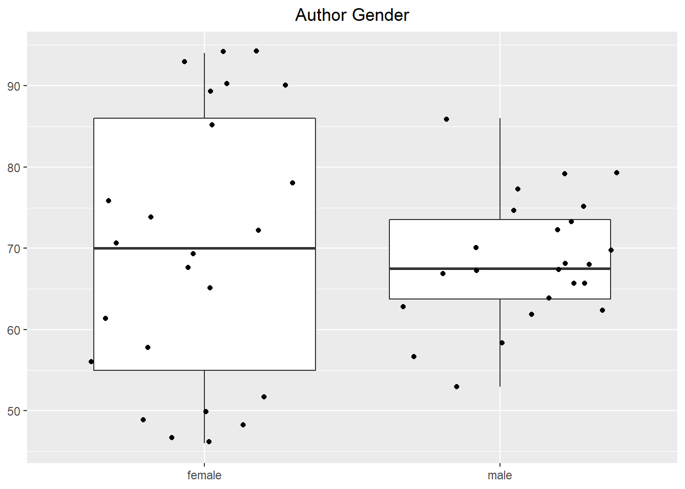
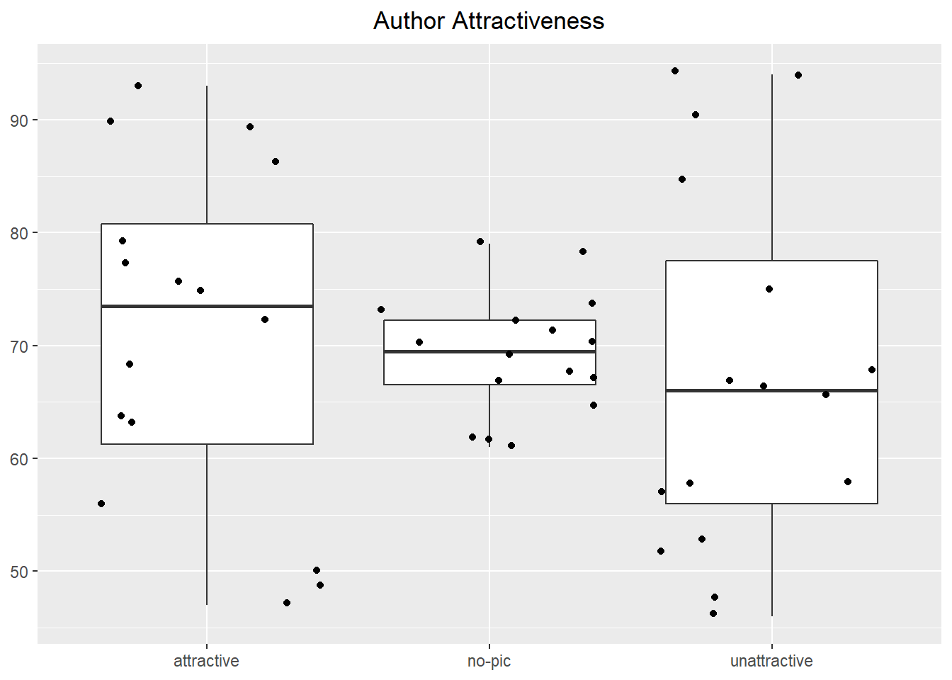
Below are some basic boxplots talent perception, grouped by levels of each experimental factor. Jittered points of the response are overlayed on each boxplot. The effect of attractiveness is detectable, but the impact of reader gender and author gender are not obvious since they exist as part of an interaction. Interaction plots can be investigated at any time in the analysis process. However, sometimes the number of interactions to check can be large, and may not be something to start with. In such cases, you may run the model first and then spend energy trying to understand only those interactions that look to be significant.
Code
#Note: the df data frame was created in the first R chunk in the Overview section of this page# Chart 1df %>%ggplot(aes(x = reader, y = talent)) +geom_boxplot(outlier.shape =NA) +geom_jitter() +labs(title ="Reader Gender") +theme(axis.title =element_blank(),plot.title =element_text(hjust = .5))# Chart 2df %>%ggplot(aes(x = author, y = talent)) +geom_boxplot(outlier.shape =NA) +geom_jitter() +labs(title ="Author Gender") +theme(axis.title =element_blank(),plot.title =element_text(hjust = .5))# Chart 3df %>%ggplot(aes(x = attractiveness, y = talent)) +geom_boxplot(outlier.shape =NA) +geom_jitter() +labs(title ="Author Attractiveness") +theme(axis.title =element_blank(),plot.title =element_text(hjust = .5))
(a)
(b)
(c)
Figure 2: Graphical Summaries of Experimental Factors
Create the Model
The 3-way Basic Factorial model is created in R just as the 2-way model was: using the aov() function. To see results of the F-test you can feed your model into a summary() or anova() function.
myaov is the user defined name in which the results of the aov() model are stored
Y is the name of a numeric variable in your dataset which represents the quantitative response variable.
X1, X2, and X3 are names of qualitative variables in your dataset. They represent the independent variables in the study. They should have class(X) equal to factor or character. If that is not the case, use factor(X) inside the aov(Y ~ factor(X1)*...) command.
YourDataSet is the name of your data set.
The * in the code above is a shortcut for writing out the whole model. It can be read as, “include each term by itself, and all possible interaction terms”. The long way of writing out the model uses a colon, :, to define interaction terms and is shown below. When writing it this way each term must be explicitly stated.
Figure 3 shows the results for the full BF[3] model for the study of halo effect on perception of talent. The 3-way interaction is significant here (p-value - 1.081e-7). Two of the two-way interactions are significant. None of the main effects show significance.
When a significant interaction is discovered, all lower order interactions and main effects should remain in the model - even if they are not significant.
When a 2-way interaction is found to be significant, then both of the simple factors (or main effects factors) should be included in the model. If a 3-way interaction is found to be significant, then the 3 main effects and all corresponding 2-way interactions should all be included in the ANOVA model - even if they are not statistically significant.
Interpreting lower order interactions and main effects in the presence of a significant higher order interaction should be done with caution. One should investigate the interaction plots in order to describe how the effect of one variable may depend on the value of another. Simply comparing marginal means2 and interpreting main effects is not sufficient and may lead to incorrect conclusions.
In this example, we will not interpret any of the main effects or two-way interactions alone, since the 3-way interaction is significant. In the Interaction section of this page, an interpretation of the interaction was already discussed. To recap that section, we saw in Figure 1 that for male readers, attractiveness of author tended to correspond to higher perceptions of talent of the author - regardless of the author’s gender. However, for female readers, the impact of author attractiveness depended on author gender: attractive female authors were perceived as less talented than unattractive female authors, whereas attractiveness had negligible effect on perceived talent of male authors.
In order to trust these hypothesis test results we need to verify that ANOVA model assumptions are met.
Check Assumptions
For a more detailed explanation of the code, output, and theory behind these assumptions visit the Assumptions page.
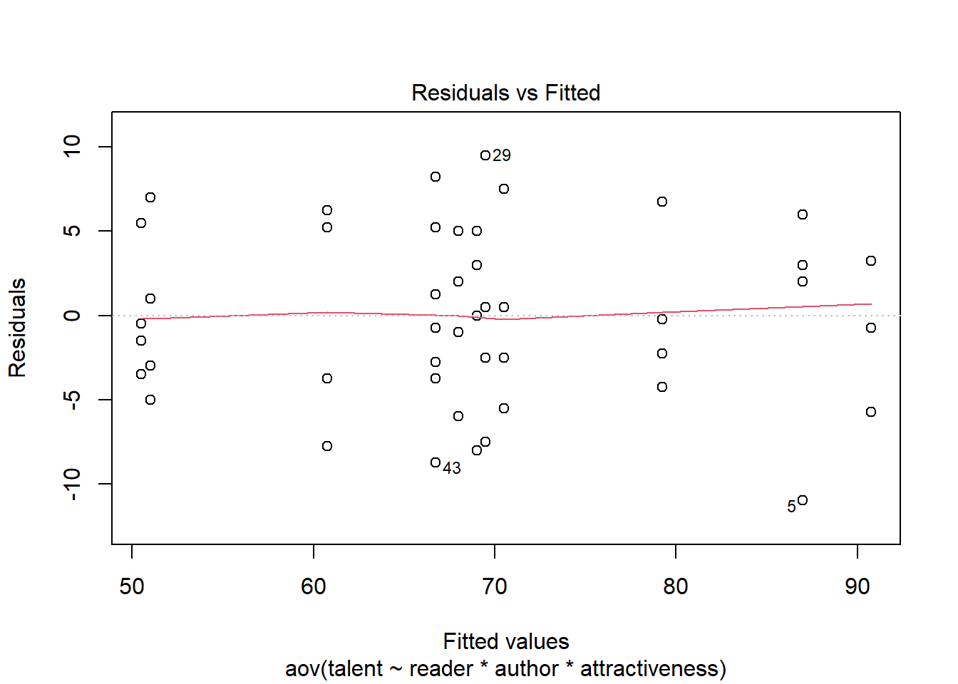
Constant Variance of Residuals
There needs to be constant variance of residuals across the factor level combinations. First, we can check the residual plot.
Code
plot(halo_aov, which =1)
Figure 4: Checking constant variance
In the residual plot, Figure 4, the vertical spread of the points is roughly constant as one moves from left to right across the x-axis of the plot. It is clear that the assumption of constant variance of the residuals is met.3 Rarely does a plot look better than this.
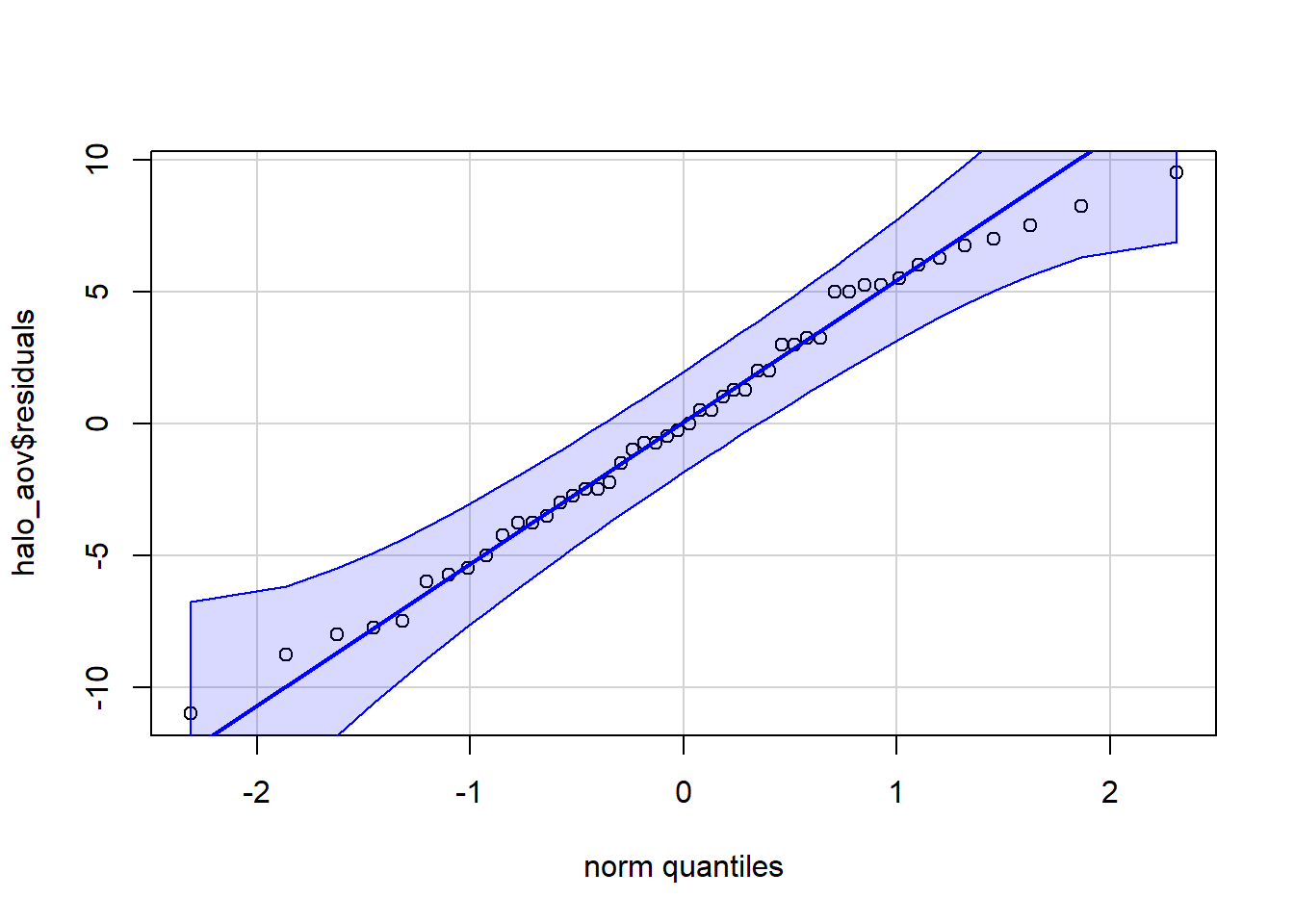
Normally Distributed Residuals
We check the assumption that residuals are normally distributed in Figure 5. All the points are in the shaded region, so we conclude this assumption is met.
Code
car::qqPlot(halo_aov$residuals, id =FALSE)
Figure 5: Checking normality of residuals
Independent Residuals
The dataset we are analyzing does not include information about the order in which the data was collected. Independence of observations often becomes a concern when there is re-use of equipment, researcher(s) making multiple measurements over time, or any other process that is repeated in each experimental run. Those types of situations can lead to order bias, which can make residuals time/order dependent rather than independent.
Nothing in this experiment suggests a potential for order bias. If we assume that random selection of participants has taken place, and that participants have randomly been assigned to treatments as indicated, there is little reason to doubt that observations (and consequently residuals too) are independent. There is no need to provide a plot in this case.
Assumptions Summary
Rarely are assumptions so clearly and obviously met. In this case, the data was simulated in order to replicate effects and interactions similar to what the original study found. Real data does not usually behave as nicely as simulated data.
The assumptions appear to be met, meaning the p-values should be valid and reliable.
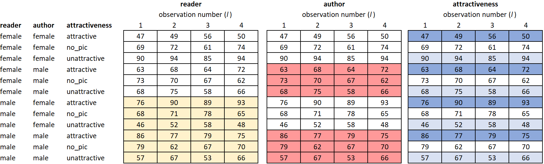
Appendix
Partitioning of the dataset that corresponds with the 7 structural factors in the 3 factor model.
Figure 6: Data Partition for Single Factors
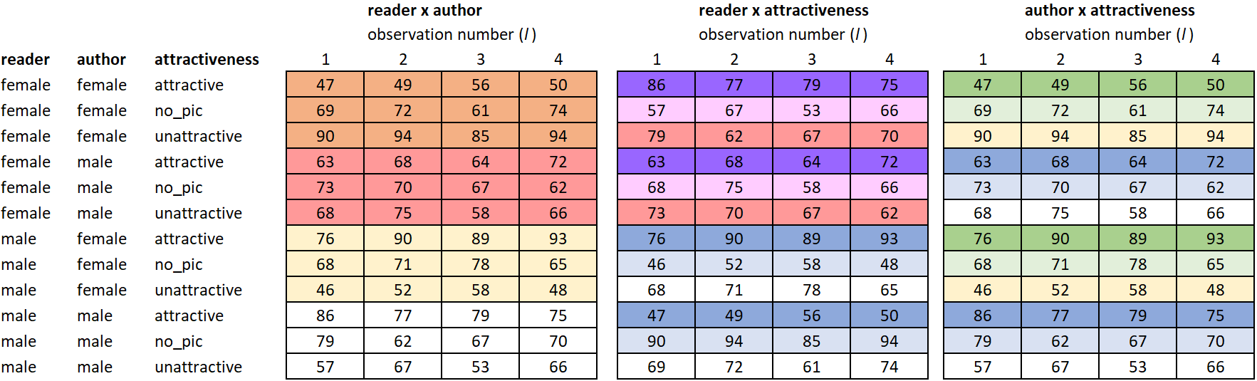
Figure 7: Data Partition for 2-Way Interaction Factors
Figure 8: Data Partition for 3-Way Interaction Factor
Footnotes
This assumes a balanced design. Formulas/calculations for unbalanced designs may need adjustments, depending on the sum of square type that is desired.↩︎
A marginal mean is a mean calculated in the “margins” (or on the endges) of a two-way table. In other words, it is a mean of a factor level without considering the other factors in the model. Stated another way, it is averaging over all the observations that belong to reader=Male, without breaking out the observations into separate groups to account for the author’s gender.↩︎
If it was questionable, Levene’s test may help with the decision of whether the assumption was met or not. In reality though, this is about as nice of a residual plot as one could hope for.↩︎