ANCOVA

ANOVA vs. Regression

So far, we have only considered experiments that use categorical factors as independent variables, and a quantitative response. It is not hard to imagine scenarios where quantitative variables serve as the independent variable. This type of analysis, where the response and the independent variable(s) are both quantitative is called regression. Students can get a review of simple linear regression from the freely available BYU-Idaho Math221 textbook. A deeper dive can be found in the BYU-Idaho Math325 textbook under Multiple Regression.

If a combination of categorical and quantitative variables are used to predict a quantitative response it could be called ANOVA or regression. Both terms are used to describe an approach or application of the generalized linear model.

In reality, the main difference between regression and ANOVA is the vocabulary associated with them and the paradigm or perspective the researcher has. The ANOVA technique originated in the early 1900’s by Ronald Fisher. It’s initial use was primarily agricultural experiments and independent variables were categorical.

Regression has been around much longer. It incorporates categorical variables through dummy coding.

Though the underlying linear algebra for both techniques is the same and the same results can be obtained regardless of the technique, the paradigm, purpose, or vocabulary for selecting a tool tends to differ. Historical precedence and inertia is driving much of the researcher’s paradigm, purpose and vocabulary.

Why not just do away with ANOVA if they are fundamentally the same? There are some that argue ANOVA provides a valuable way to describe, to teach, and to talk about how variables are related. In particular, ANOVA can be useful for “summarizing complex high-dimensional inferences and for exploratory data analysis”. For a brief introduction to the discussion, you can read this exachange..

ANOVA is used in this text for its “ease of teaching/applying the tool”¹ (especially to a non-statistician audience) and to prepare students for the vocabulary many of them will encounter in their field. These same students should also seek exposure to regression and the generalized linear model.

Choosing a Covariate

In ANCOVA, we explore the introduction of a quantitative explanatory variable to the ANOVA model. This quantitative variable is also called a concomitant variable, or a covariate. It is considered a nuisance variable because it is not the main focus of the study, but potentially can account for a substantial amount of variation in the response. The covariate should correlate with the response, but should NOT be influenced by the treatment.

ANCOVA is a good technique when the nuisance covariate cannot be controlled or cannot be measured until the time the experiment is being conducted. ANCOVA also comes in handy when new sources of variation come to mind after the experiment has already been executed, as in the following example.

Example: Benefits of ANCOVA

A company wanted to study how distributing a coupon could effect sales. The company randomly selected 4 stores and distributed coupons for those stores. For another 4 stores the company would not distribute coupons, but would still track sales.

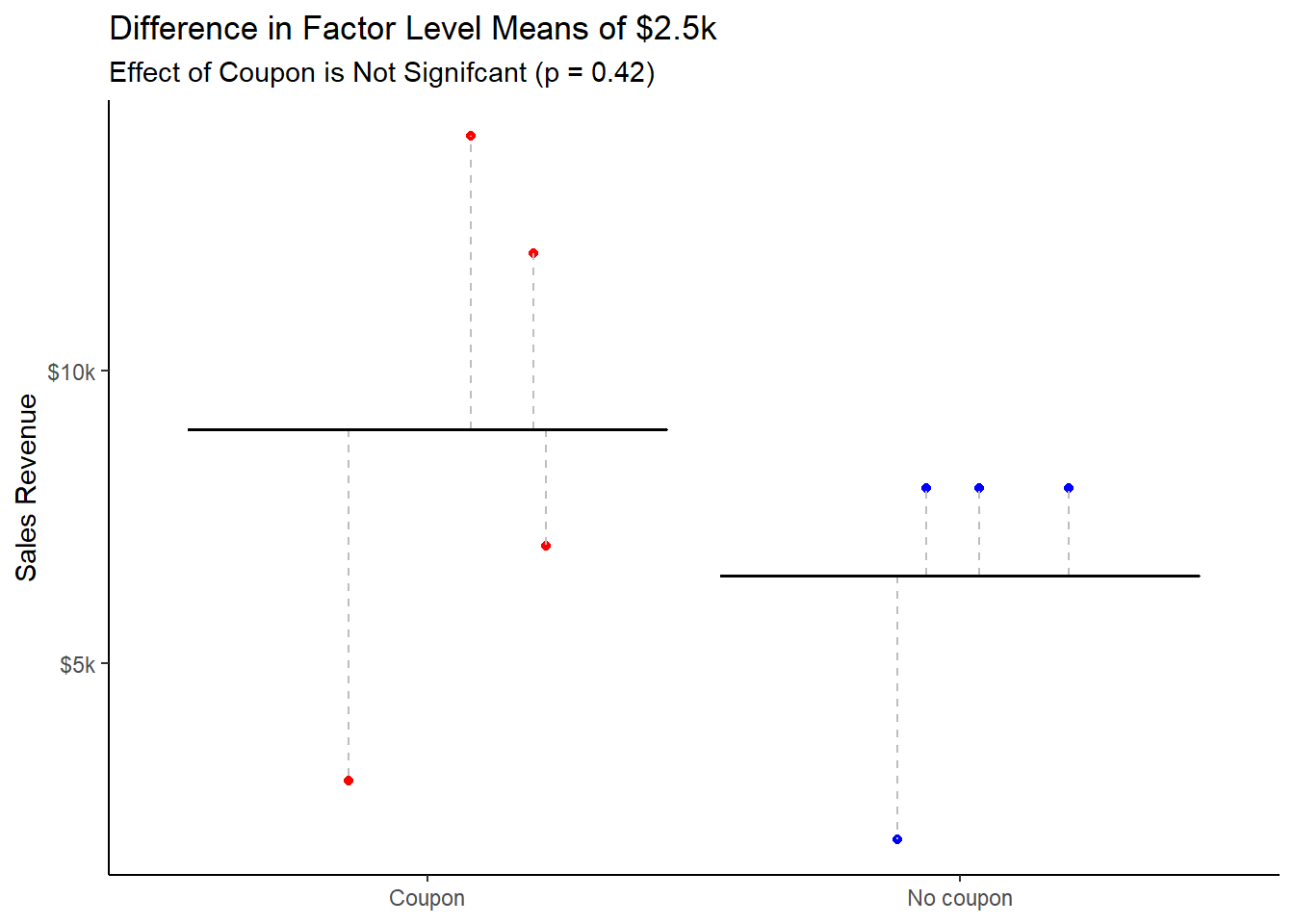
Initial analysis of the results, contained in Figure 1 (a), surprised the company. The difference in mean sales between the coupon group and the non-coupon group was small (only $2,500) relative to the variability within each group. A hypothesis test of the difference revealed no statistically significant results.

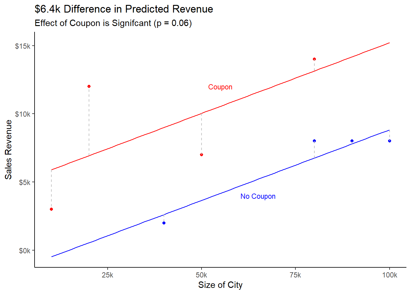
The company’s BYU-Idaho intern realized that the research team had not accounted for the fact that some stores were in smaller cities than others. He noticed that the “no coupon” stores tended to be located in larger cities, with potential for more sales. The “coupon” group of stores tended to be located in smaller cities. This can be seen in Figure 1 (b), notice the “no coupon” group tends to be located farther to the right on the x-axis.

The relationship between city size and sales revenue was accounted for with a regression line for each group (see Figure 1 (b)). Researchers adjusted for the difference in city size between the two groups and found the difference in predicted revenue between “coupon” and “no coupon” groups was actually $6,400. This difference is considered significant at the \(\alpha = 0.10\) level.

(a)

(b)

Figure 1: Benefit of a Covariate

Notice the straight, parallel lines in panel (b) of the above plot. This is a visual indicator that there is no interaction between the covariate and the independent treatment factor. In other words, the effect of the treatment does not change depending on the value of the covariate (city size).

Situations where there is a significant interaction between the coviarate and the treatment factor are valid and common. However, when an interaction is present, the situation is generally called regression rather than ANCOVA.

There are a couple key advantages to using a covariate in the analysis. Much like blocking, a covariate can reduce mean squared error; thereby increasing our ability to detect a significant treatment effect. It can also reduce bias caused by differences in treatment groups, as we saw in the coupon example above.

Beware of using ANCOVA to adjust for differences in groups of observational data. Doing so may require you to extrapolate from the line to a region where there are no (or few) observations. Consider a study that investigated the effect of a fertilizer on two types of trees: palm trees and pine trees. Researchers also considered the effect that air temperature could have on the way the fertilizer worked. They randomly selected nurseries from across the state of California to participate in the study. The nurseries applied the fertilizer to a mature tree and then measured the growth after 12 months.

The covariate in this case is the temperature of the surrounding area. The factor is the tree type (it is an observational factor, not an experiment). The problem lies in the fact that palm trees are all found in a warmer climate and the pine trees tend to be found in cooler climate. It is not appropriate to extrapolate the relationship of temperature and growth to predict how either tree would do in the other climate since we don’t have data in those conditions.

In addition, the covariate value should not be affected by the treatment. Nor should the covariate effect the random assignment. This is an experimental design assumption, not an analysis assumption. If you were doing an observational study, random assignment does not occur, and the ANCOVA analysis can be quite help in isolating the effect of each variable in the presence of the other. In an observational study you could commonly see correlation between an independent factor and a continuous covariate.

ANCOVA vs. Blocking

In the coupon example above, if the researchers had thought of it in advance, the random assignment of coupon to store could have been blocked based on city size. If either technique could be employed, which one should you choose?

Blocking is Preferred

If it makes sense to do so, blocking is preferred. Good design is preferred over using analysis techniques to compensate / correct for poor design. A good design can lead to good analysis.

Blocking is preferred because its requirements are less stringent. Blocking does not require you to specify the nature of the relationship between the response and the covariate. In ANCOVA you are required to explicitly model the relationship between the response and the covariate (linear, quadratic, etc.). The effectiveness of ANCOVA will depend on how well that relationship is modeled and whether it is reasonable to use the same slope for both groups. Generally, it is better to prevent having bias in group compositions than adjusting for it afterward in the analysis.

Though blocking is generally preferred over ANCOVA, there are valid reasons for doing ANCOVA instead. Blocking requires you to have values on the covariate in advance - during the design phase. This may be difficult or impossible to do. ANCOVA is more flexible in this regard, covariate values can be collected during or even after execution of the experiment.

In other cases the treatment cannot truly be assigned and so an observational study is conducted. Without the ability to assign treatments, a blocked design may not be feasible and ANCOVA will be needed.

Design

The ANCOVA analysis technique can be applied to a completely randomized design or observational study data.

Model and Hypotheses

The ANCOVA model is written as:

\[ y_{ij} = \mu + \alpha*x_i + \beta_j + \epsilon_{ij} \tag{1}\]

Where

• \(y_{ij}\) represents the observations. i is a unique ID number for every row in the dataset. j indicates what level of \(\beta\), the treatment factor, that individual received.

• \(\mu\) is the grand mean of the entire dataset. (This can also be thought of as the y-intercept of a “common line” where no treatment effects are present.)

• \(\alpha\) is the slope of the line. It is the change in the expected value of y for every 1 unit change in x.

• \(x_i\) is the value of the covariate for individual i.

• \(\beta\) is the effect of treatment factor, which has j levels.

• \(\epsilon\) is the residual error term

The hypothesis of interest for a simple ANCOVA model is about the treatment factor:

\[H_0: \beta_j = 0 \text{ for all }j\]

\[H_a: \beta_j \ne 0 \text{ for some }j\]

To be sure the ANCOVA model is appropriate, the researcher should test for an interaction between the treatment factor and covariate. If the interaction is significant, the researcher should proceed to a regression analysis with the interaction term included. If the interaction term is NOT significant, the simpler ANCOVA model (Equation 1) can be adopted.

“Unfortunately, the hypothesis test we have used previously for balanced designs does not work in this case. The covariate values are not balanced in relation to the rest of the design.”² Practically speaking this means we cannot use the Type I Sums of Squares (SS) and must use a different type instead, likely a Type III SS.

To read an explanation on how an F Test for treatment is calculated click here

The F test for the treatment factor in the Type III SS represents a ratio of squared errors. The denominator contains the mean squared error (MSE) for the “full” model: the model described by Equation 1.

In contrast to the full model, the reduced model is the model obtained by ignoring treatment effects. In other words, it is a simple linear regression between the response and the covariate. This is the model we would get if the null hypothesis for the treatment factor were true.

To get the F statistic for treatment you must first calculate the difference in Sum of Squared Error between the full and reduced models. In other words, how much did the Sum of Squared Error change by adding the treatment factor to the model. The difference in Sum of Squared Error is then divided by the difference in degrees of freedom for error between the full and reduced model.

The numerator degrees of freedom for this F test statistic is calculated as the number of levels in the treatment factor minus one. The denominator degrees of freedom is equal to the degrees of freedom for error under the full model.

\[ F_\text{treatment factor} = \frac{ \frac{SSE_\text{reduced} - SSE_\text{full}} {df\text{ error}_\text{reduced} - df\text{ error}_\text{full}}} {MSE_\text{full model}} \]

To summarize at a high level, the treatment factor F statistic is a ratio of the reduction in unexplained variance over the unexplained variance that remains in the model when the treatment factor is included. In other words, was the amount of variance explained by the treatment vary large relative to the total error variance? Stated this way, we can recognize that the F test interpretation has not changed.

Though the formula may seem a little different, the good news is that R will do these calculations quickly and seamlessly without requiring a change in how we interpret the ANOVA summary table.

Assumptions

The assumptions for the ANCOVA model are essentially the same as for CB[1], with the addition that the response and the covariate need to have a linear relationship:

Requirements	Method for Checking	What You Hope to See
Linear relationship between covariate and response	Residual vs. Fitted Plot	No trend or pattern
Constant variance across factor levels	Residual vs. Fitted Plot	No wedge or megaphone shape
Normally Distributed Residuals	Normal Q-Q plot	Straight line, majority of points in boundaries
Independent residuals	Order plot (only if applicable)	No pattern/trend
	Familiarity with/critical thinking about the experiment	No potential source for bias

The following example illustrates how to conduct an ANOVA in R.

Analysis in R

Biggest Loser is a reality TV show where contestants try to lose as much weight as possible in a certain number of weeks. We are interested in using a dataset containing information about Biggest Loser contestants to generalize to the broader population. The dataset contains information about all contestants during the first 17 seasons. Specifically, we are interested in whether a person’s age group has a significant effect on their weight loss. We will define the age groups as

• Youngest (<35 years old)
• Middle, Young (35-49 years old),
• Oldest (>50 years old)

It is believed that people with a higher starting weight will find it easier to loose a larger proportion of their weight. Therefore, a person’s starting weight (measured in pounds) will be used as a covariate.

First we load required packages, read in the data, and store the age group information in a variable called ymo.

#You can read in the data with this path directly from the web:
# https://byuistats.github.io/Math326_Quarto4/data/biggest_loser_ancova.csv

bl_data <- read_csv("data/biggest_loser_ancova.csv") %>% 
  select(prop_initial_weight_lost, initial_weight_at_start_show, contestant_age) %>% 
  mutate(ymo = case_when(contestant_age < 35 ~ "Youngest",
                                                contestant_age < 50 ~ "Middle",
                                                contestant_age >= 50 ~ "Oldest"),
         ymo = factor(ymo, levels = c("Youngest", "Middle", "Oldest")))

Describe the Data

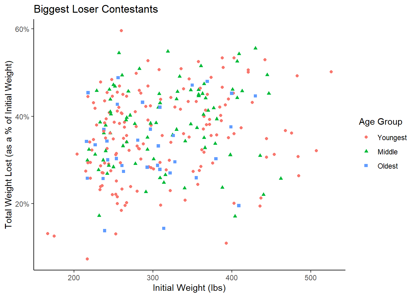
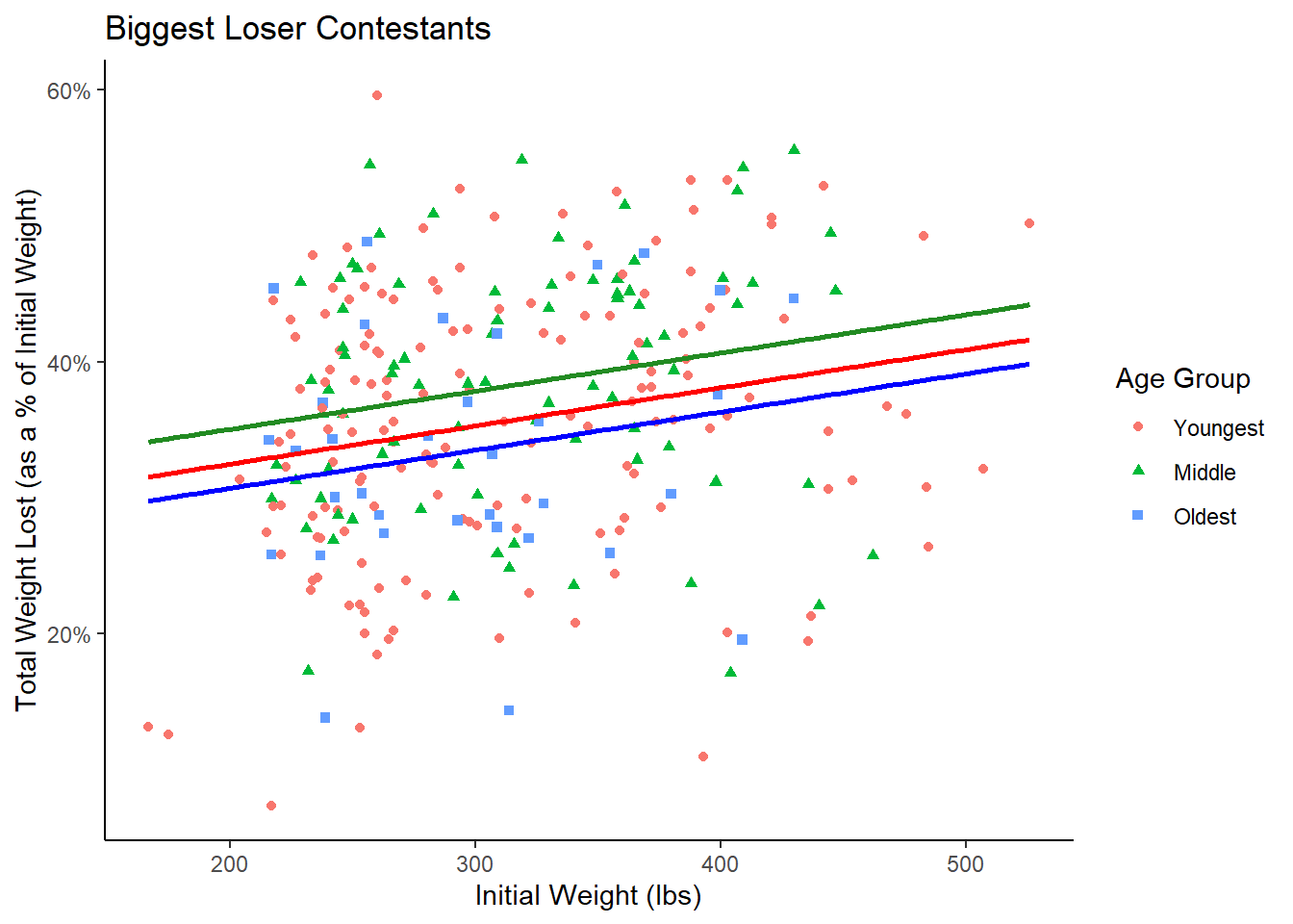
A scatterplot of the proportion of initial weight lost and initial weight is presented below, with each point colored according to their age group. A numeric summary of the data by age group is also presented.

bl_data %>% 
  ggplot(aes(x = initial_weight_at_start_show, y = prop_initial_weight_lost,
             color = ymo, shape = ymo), size = 3) +
  geom_point()  +
  theme_classic() + 
#  theme(legend.position = "top") +
  scale_y_continuous(labels = scales::label_percent(scale = 1)) +
#  scale_shape_manual(values = c(16, 17, 18))+
  labs(y = "Total Weight Lost (as a % of Initial Weight)", x = "Initial Weight (lbs)", title = "Biggest Loser Contestants", color = "Age Group", shape = "Age Group")
#  geom_smooth(method = "lm", se = FALSE)

Figure 2: Graphical Summary

favstats(initial_weight_at_start_show~ymo, data = bl_data) %>% select(-missing) %>% pander()
favstats(prop_initial_weight_lost ~ ymo, data = bl_data) %>% select(-missing) %>% pander()

Table 1: Numerical Summary by Age Group

(a) Initial Weight (lbs)

ymo	min	Q1	median	Q3	max	mean	sd	n
Youngest	167	252.5	289.5	367.2	526	311	75.48	160
Middle	217	254.5	309	365	462	317.3	65.99	83
Oldest	216	245.8	295	327.5	430	298.1	60.61	34

(b) Percent of Initial Weight Lost

ymo	min	Q1	median	Q3	max	mean	sd	n
Youngest	7.37	28.98	35.84	43.24	59.62	35.6	9.952	160
Middle	17.08	31.68	38.63	45.41	55.58	38.34	9.057	83
Oldest	13.81	27.95	33.35	40.95	48.83	33.46	9.035	34

The scatterplot and table make it apparent that the Oldest group tends to loose a smaller percentage of their initial weight than their older counterparts. Furthermore, the maximum and the mean initial weight of Oldest contestants is lower than the maximum and mean initial weight of the other two age groups respectively.

Create and Test the Model

Generic Code

Create the model using the lm() function.

cov_mod <- lm(Y ~ covariate + treatment, 
              data = YourDataSet, 
              contrasts = list(treatment = contr.sum))

• cov_mod is the user defined name in which the results of the aov() model are stored
• lm stands for linear model. It is like an aov object, but it is better suited to working with models that have continuous covariates (i.e. continuous independent variables) , rather than strictly factors.
• Y is the name of a numeric variable in your dataset which represents the quantitative response variable.
• covariate is the name of the covariate in your dataset.
• treatment is the name of the controlled factor in your dataset. It should have class() equal to factor or character. If that is not the case, use factor(X) inside the lm(Y ~ factor(treatment)...) command.
• contrasts is an argument that allows you to specify how factor variables should be set-up in R. When dealing with factor variables, R actually changes each factor variable into a group of “dummy” variables to represent the individual factor levels. The default contrast in R does not work well with the Type 3 sums of squares, which is what we need when working with continuous covariates. Therefore, we specify a different contrast. The term contrast is referring to the columns in the X matrix that are used to represent the dummy variables.
• YourDataSet is the name of your data set.

The model above assumes that the interaction between the covariate and the treatment factor is zero. Rather than assuming that is the case, it is advisable to include the interaction term in the model and test the significance of the interaction. If the interaction is NOT significant it can be removed; if it is significant, then it should remain in the model. To include the interaction in the model the following code would be used. Remember that if an interaction is significant, interpreting the main effects should only be done with great care.

cov_mod <- lm(Y ~ covariate + treatment + covariate:treatment, 
              data = YourDataSet,
              contrasts = list(treatment = contr.sum))

After creating the model, results of the hypothesis tests for each term in the model can be seen using the Anova() command from the car package. Don’t forget to specify type = 3 in the Anova() command, since a Type 1 Sum of Squares is not appropriate when a covariate is in the model.

library(car)
Anova(cov_mod, type = 3)

Code for checking model assumptions is found on the diagnostics page, under the “R Instructions” menu of this book.

Biggest Loser

We first create the model, with proportion of initial weight lost as the response, initial weight (in pounds) as the covariate, and age group as our factor of interest. We will also include the interaction between initial weight and age group in the model to see if it is significant.

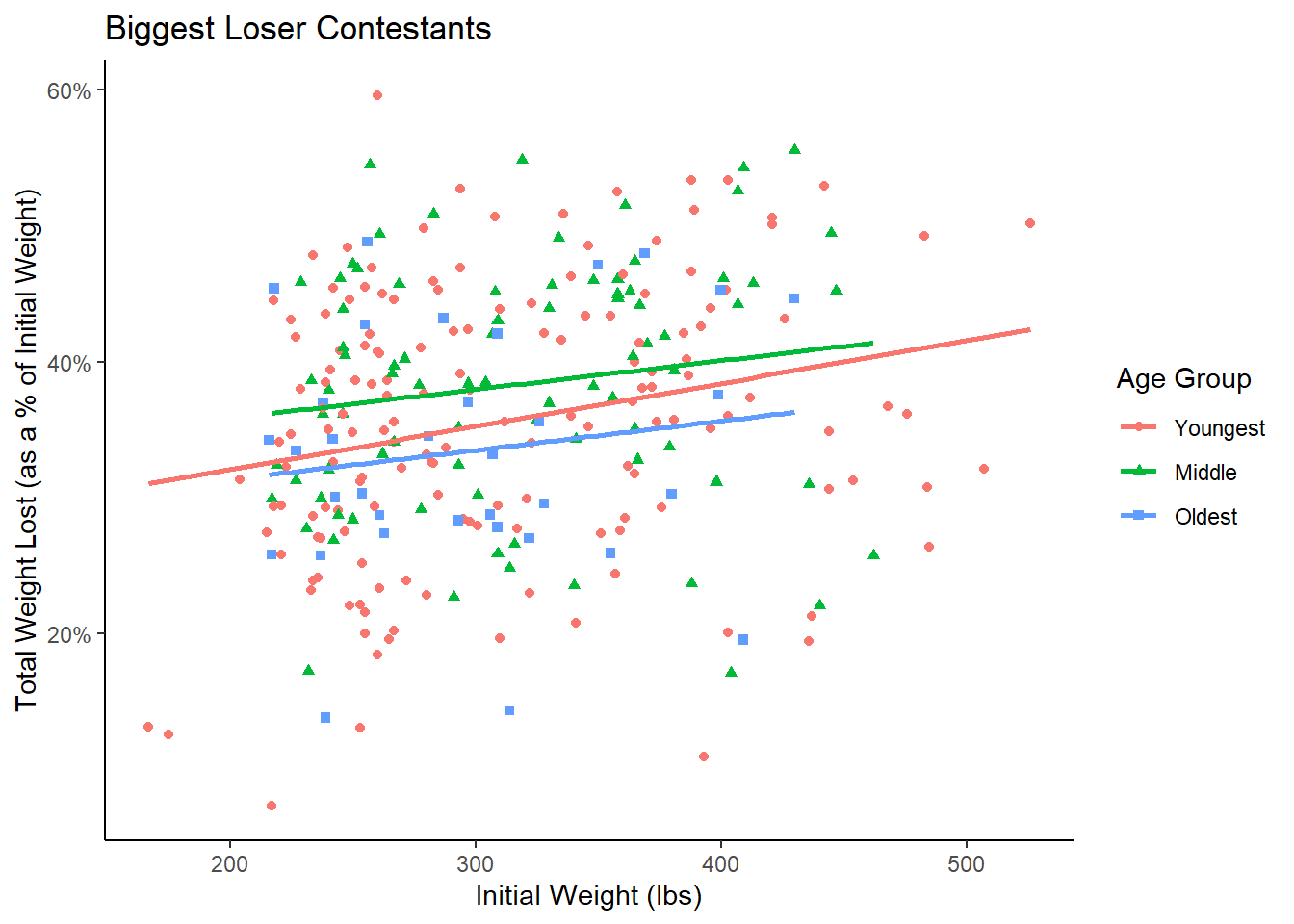
This model equates to fitting a separate best-fit line for each group, each line having the potential for a unique slope - as depicted in Figure 3.

Figure 3: Interaction Term Included Allows for Unique Slopes

The slope of the lines for Middle and Oldest appear nearly identical. The slope for Youngest appears different, but we will create the model and run the hypothesis test on the interaction term to be sure.

bl_data2 <- bl_data %>% rename(`Age groups` = ymo, `Initial weight` = initial_weight_at_start_show)

bl_mod_with_interaction <- lm(prop_initial_weight_lost ~ `Initial weight` + `Age groups` + `Initial weight`:`Age groups`, 
                              data = bl_data2,
                              contrasts = list(`Age groups` = contr.sum))

pander(Anova(bl_mod_with_interaction, type = 3))

Anova Table (Type III tests)

	Sum Sq	Df	F value	Pr(>F)
(Intercept)	6090	1	68.65	5.477e-15
Initial weight	455.8	1	5.138	0.0242
Age groups	84.36	2	0.4755	0.6221
Initial weight:Age groups	33.6	2	0.1894	0.8276
Residuals	24042	271	NA	NA

With a p-value of 0.8276, there is insufficient evidence to claim the interaction is not zero. We therefore remove it from the model and proceed with the analysis.

Note

Do not forget to verify the model requirements are met before trusting the conclusion that the interaction term is not significant. This can be done with plot(bl_mod_with_interaction, which = 1:2).

The ANCOVA model (i.e. covariate included without an interaction term) is created.

ymo_ancova <- lm(prop_initial_weight_lost ~ `Initial weight` + `Age groups`, 
                  data = bl_data2,
                 contrasts = list(`Age groups` = contr.sum))

The model is graphically depicted in Figure 4.

Figure 4: ANCOVA, Equal Slopes Model

The hypothesis test for the treatment factor is

\[H_0: \beta_\text{Youngest} = \beta_\text{Middle} = \beta_\text{Oldest} = 0\]

\[H_a: \beta_j \ne 0 \text{ for some }j \in \{\text{Youngest, Middle, Oldest}\}\]

We will use a significance level of \(\alpha = 0.05\).

The results of the ANOVA test are shown below.

pander(Anova(ymo_ancova, type = 3))

Anova Table (Type III tests)

	Sum Sq	Df	F value	Pr(>F)
(Intercept)	9920	1	112.5	3.113e-22
Initial weight	1091	1	12.37	0.00051
Age groups	566	2	3.209	0.04193
Residuals	24075	273	NA	NA

summary provides a different set of output, but does not include an F test for the factor. Rather, it provides unadjusted t-tests of whether each factor level mean is equal to the mean of the reference factor level’s mean.

The p-value for age groups is .04193, which is lower than our significance level. This means that, after accounting for the impact of a person’s initial weight, the person’s age group has a significant effect on proportion of weight lost. From Figure 4, we see that the Middle group (green line) and Young roup (red line) seem to loose a higher percentage of weight, while the Oldest (blue line) tends to loose less.

Incidentally, the low p-value (p = .00051) associated with Initial weight is an indicator that there is a significant relationships between the response variable and Initial weight. Therefore, initial weight is probably important to keep in the model.

Notice that with the first model, the interaction term was included but was non-significant. When it was included, the other terms were also non-significant. The interaction term seemed to be hiding the significance of the other variables. Removing it allowed us to uncover the true relationships between the variables. It is important to include the right terms in your model rather than blindly leaving everything in. The process of model building is a complicated topic and a whole course could be dedicated to it. The purpose of this discussion is simply to point out that selecting the right terms of the model is important.

Check Assumptions

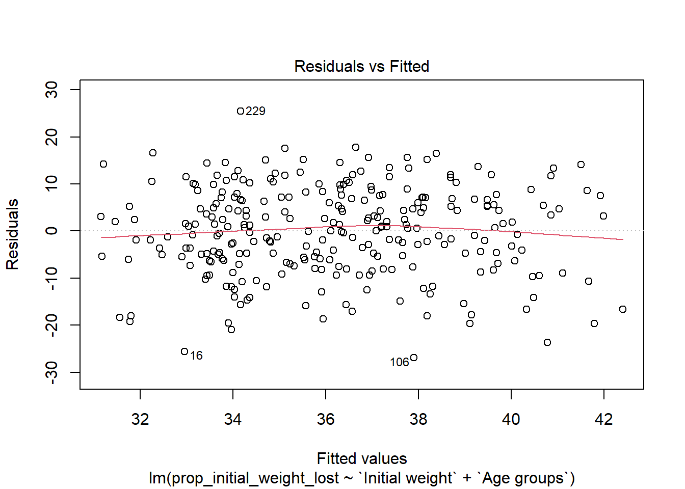
The first two assumptions (linear relationship of response and covariate, and constant variance of the error term) can be checked with a residual vs. fitted plot. If the plot appears to be a random scatter with no patterns or trends, then both assumptions are considered met.

plot(ymo_ancova, which = 1)

Figure 5

Linear Relationship Between Response and Covariate

To verify the response variable and the covariate have a linear relationship we check the residual vs. fitted plot, Figure 5. No major patterns or trends or evident so we consider this assumption satisfied.

In addition, R adds the red line to the plot. The red line is very flat, an additional indicator the assumption is met. Sometimes, when sample sizes are small, the red line can be confusing. In the case of small sample sizes the red line becomes very sensitive and bounces around a lot - becoming more of a distraction than an aid.

Constant Error Variance

To verify that the assumption of a constant error term is valid, the residual vs. fitted plot should not show trends or patterns. In particular, if the points in the residual vs. fitted plot created a megaphone, wedge, or triangle shape we would conclude this assumption is violated. In other words, instead of having constant variance, the vertical spread of the points on the plot increase (or decrease) as you move from the left to the right side of the plot. Since Figure 5 does not have this problem, the constant error variance assumption is considered met.

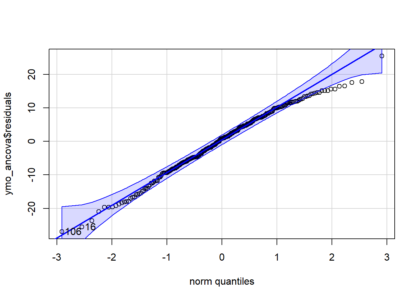
Normally Distributed Error Term

We check the assumption that residuals are normally distributed with a QQ plot. The QQ plot below shows there may be some skew to the residuals. The points on the right side of the plot are trending away from the line and outside of the shaded bounds. The skew does not appear to be severe however, and if the other assumptions are solidly met, we may continue to use the model output as is.

car::qqPlot(ymo_ancova$residuals)

[1] 106  16

Independent Residuals

This assumption is not easily checked with the data. Usually, an understanding of how the data was generated and what it represents is the best way to check this assumption. With some research about the show, one can come to know that each observation comes from a particular season. In each season, the contestant is assigned to 1 of 2 trainers (or 1 of 2 teams of trainers). Thus, contestants belonging to the same season and the same trainer may have residuals that are related. Plots of residuals by trainer within a season may reveal patterns in the data. If a plot of residuals by trainer/season looks like a random scatter then we can feel assured this assumption is met. If a trend is discovered, we will want to somehow incorporate trainer/season into the model.

As you can see, some expert judgement and understanding of context will drive you to know which variables are worth investigating or could threaten the independence assumption.

Assumptions Summary

Aside from the potential violation of independent residuals, the diagnostic plots look good enough to trust the model results.

Footnotes

1. https://stats.stackexchange.com/questions/555/why-is-anova-taught-used-as-if-it-is-a-different-research-methodology-compared

2. George W. Cobb. Introduction to Design and Analysis of Experiments. Wiley, 2014. pp 681.