A nonparametric approach to computing the p-value for any test statistic in just about any scenario.


Overview

In almost all hypothesis testing scenarios, the null hypothesis can be interpreted as follows.

\(H_0\): Any pattern that has been witnessed in the sampled data is simply due to random chance.

Permutation Tests depend completely on this single idea. If all patterns in the data really are simply due to random chance, then the null hypothesis is true. Further, random re-samples of the data should show similar lack of patterns. However, if the pattern in the data is real, then random re-samples of the data will show very different patterns from the original.

Consider the following image. In that image, the toy blocks on the left show a clear pattern or structure. They are nicely organized into colored piles. This suggests a real pattern that is not random. Someone certainly organized those blocks into that pattern. The blocks didn’t land that way by random chance. On the other hand, the pile of toy blocks shown on the right is certainly a random pattern. This is a pattern that would result if the toy blocks were put into a bag, shaken up, and dumped out. This is the idea of the permutation test. If there is structure in the data, then “mixing up the data and dumping it out again” will show very different patterns from the original. However, if the data was just random to begin with, then we would see a similar pattern by “mixing up the data and dumping it out again.”

The process of a permutation test is:

  1. Compute a test statistic for the original data.
  2. Re-sample the data (“shake it up and dump it out”) thousands of times, computing a new test statistic each time, to create a sampling distribution of the test statistic.
  3. Compute the p-value of the permutation test as the percentage of test statistics that are as extreme or more extreme than the one originally observed.

In review, the sampling distribution is created by permuting (randomly rearranging) the data thousands of times and calculating a test statistic on each permuted version of the data. A histogram of the test statistics then provides the sampling distribution of the test statistic needed to compute the p-value of the original test statistic.


R Instructions

Any permutation test can be performed in R with a for loop.

#Step 1 Compute a test statistic for the original data.
myTest <- …perform the initial test… This could be a t.test, wilcox.test, aov, kruskal.test, lm, glm, chisq.test, or any other R code that results in a test statistic. It could even simply be the mean or standard deviation of the data.
observedTestStat <- …get the test statistic… Save the test statistic of your test into the object called observedTestStat. For tests that always result in a single test statistic like a t.test, wilcox.test, kruskal.test, and chisq.test it is myTest$statistic. For an aov, lm, or glm try printing summary(myTest)[] to see what values you are interested in using.
observedTestStat Print the value of the test statistic of your test to the screen. This is the value that we now need to use to compute the P-value from by finding the probability that a randomly computed test statistic would be “more extreme” than this originally observed value.

#Step 2 Re-sample the data (“shake it up and dump it out”) thousands of times, computing a new test statistic each time, to create a sampling distribution of the test statistic.
N <- 2000       N is the number of times you will reuse the data to create the sampling distribution of the test statistic. A typical choice is 2000, but sometimes 10000, or 100000 reuses are needed before useful answers can be obtained.
permutedTestStats <-  This is a storage container that will be used to store the test statistics from each of the thousands of reuses of the data. rep(NA, N) The rep() function repeats a given value N times. This particular statement repeats NA’s or “missing values” N times. This gives us N “empty” storage spots inside of permutedTestStats that we can use to store the N test statistics from the N reuses of the data we will make in our for loop.
for The for loop is a programming tool that lets us tell R to run a certain code over and over again for a certain number of times.  (i in   In R, the for loop must be followed by a space, then an opening parenthesis, then a variable name (in this case the variable is called “i”), then the word “in” then a list of values. 1:N The 1:N gives R the list of values 1, 2, 3, … and so on all the way up to N. These values are passed into i one at a time and the code inside the for loop is performed first for i=1, then again for i=2, then again for i=3 and so on until finally i=N. At that point, the for loop ends. ) Required closing parenthesis on the for (i in 1:N) statement. { This bracket opens the code section of the for loop. Any code placed between the opening { and closing } brackets will be performed over and over again for each value of i=1, i=2, … up through i=N.
   Two spaces in front of every line inside of the opening { and closing } brackets helps keep your code organized. permutedTest <- …perform test with permutedData… The same test that was performed on the original data, should be performed again but with randomly permuted data. The easiest way to permute data is with sample(y-variable-name) inside your test. See the Explanation tab for details.
   Two spaces in front of every line inside of the opening { and closing } brackets helps keep your code organized. permutedTestStats This is the storage container that was built prior to the for (i in 1:N) code. Inside the for loop, this container is filled value by value using the square brackets [i]. [i] The square brackets [i] allows us to access the “i”th position of permutedTestStats. Remember, since this code is inside of the for loop, i=1 the first time through the code, then i=2 the second time through the code, i=3 the third time through, and so on up until i=N the Nth time through the code.  <- …get test statistic… The test statistic from permutedTest is accessed here and stored into permutedTestStats[i].
} The closing } bracket ends the code that is repeated over and over again inside the for loop.
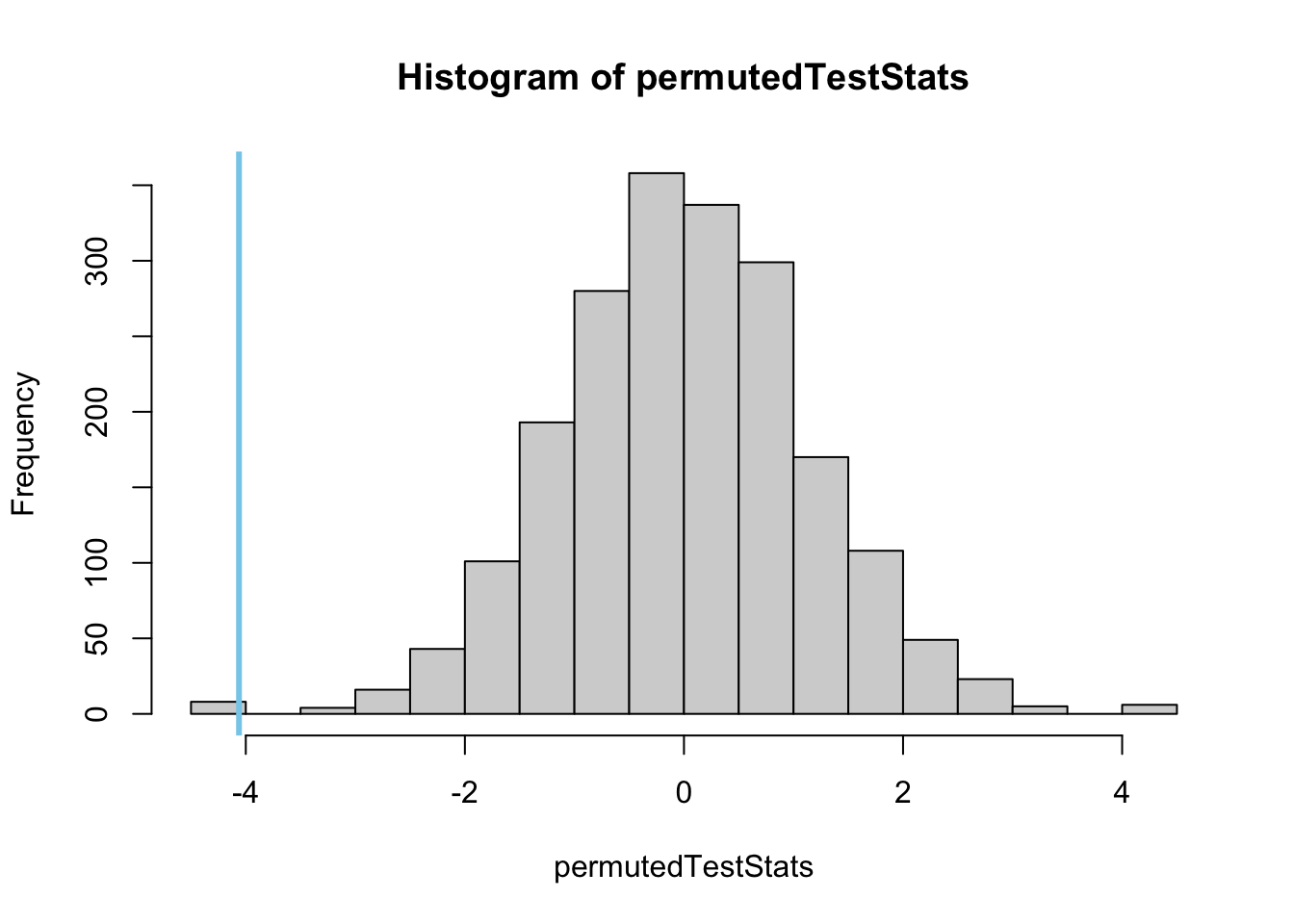
hist(permutedTestStats) Creating a histogram of the sampling distribution of the test statistics obtained from the reused and permuted data allows us to visually compare the observedTestStat to the distribution of test statistics to visually see the percentage of test statistics that are as extreme or more extreme than the observed test statistic value. This is the p-value.
abline(v=observedTestStat) This adds the observedTestStat to the distribution of test statistics to visually see the percentage of test statistics that are as extreme or more extreme than the observed test statistic value. This is the p-value.

#Step 3 Compute the p-value of the permutation test as the percentage of test statistics that are as extreme or more extreme than the one originally observed.
sum(permutedTestStats >= observedTestStat)/N This computes a “greater than” p-value. A two-sided p-value could be obtained by multiplying this value by 2 if the observed test statistic was on the right hand side of the histogram.
sum(permutedTestStats <= observedTestStat)/N This computes a “less than” p-value. A two-sided p-value could be obtained by multiplying this value by 2 if the observed test statistic was on the left hand side of the histogram.


Explanation

The most difficult part of a permutation test is in the random permuting of the data. How the permuting is performed depends on the type of hypothesis test being performed. It is important to remember that the permutation test only changes the way the p-value is calculated. Everything else about the original test is unchanged when switching to a permutation test.

Independent Samples t Test

For the independent sample t Test, we will use the data from the independent sleep analysis. In that analysis, we were using the sleep data to test the hypotheses:

\[ H_0: \mu_\text{Extra Hours of Sleep with Drug 1} - \mu_\text{Extra Hours of Sleep with Drug 2} = 0 \] \[ H_a: \mu_\text{Extra Hours of Sleep with Drug 1} - \mu_\text{Extra Hours of Sleep with Drug 2} \neq 0 \]

We used a significance level of \(\alpha = 0.05\) and obtained a P-value of \(0.07939\). Let’s demonstrate how a permutation test could be used to obtain this same p-value. (Technically you only need to use a permutation test when the requirements of the original test were not satisfied. However, it is also reasonable to perform a permutation test anytime you want. No requirements need to be checked when performing a permutation test.)

# First run the initial test and gain the test statistic:
myTest <- t.test(extra ~ group, data = sleep, mu = 0)
observedTestStat <- myTest$statistic

# Now we run the permutations to create a distribution of test statistics
N <- 2000
permutedTestStats <- rep(NA, N)
for (i in 1:N){
  permutedTest <- t.test(sample(extra) ~ group, data = sleep, mu = 0)
  permutedTestStats[i] <- permutedTest$statistic
}

# Now we show a histogram of that distribution
hist(permutedTestStats, col = "skyblue")
abline(v = observedTestStat, col = "red", lwd = 3)

#Greater-Than p-value: Not the correct one in this case
sum(permutedTestStats >= observedTestStat)/N

# Less-Than p-value: Not the correct one for this data
sum(permutedTestStats <= observedTestStat)/N

# Two-Sided p-value: This is the one we want based on our alternative hypothesis.
2*sum(permutedTestStats <= observedTestStat)/N

Note The Wilcoxon Rank Sum test is run using the same code except with myTest <- wilcox.test(y ~ x, data=...) instead of t.test(...) in both Step’s 1 and 2.

ANOVA (click to show/hide)

Simple Linear Regression (click to show/hide)