
Making Inference
It is common to only have a sample of data from some population of interest. Using the information from the sample to reach conclusions about the population is called making inference. When statistical inference is performed properly, the conclusions about the population are almost always correct.
Hypothesis Testing
One of the great focal points of statistics concerns hypothesis testing. Science generally agrees upon the principle that truth must be uncovered by the process of elimination. The process begins by establishing a starting assumption, or null hypothesis (\(H_0\)). Data is then collected and the evidence against the null hypothesis is measured, typically with the \(p\)-value. The \(p\)-value becomes small (gets close to zero) when the evidence is extremely different from what would be expected if the null hypothesis were true. When the \(p\)-value is below the significance level \(\alpha\) (typically \(\alpha=0.05\)) the null hypothesis is abandoned (rejected) in favor of a competing alternative hypothesis (\(H_a\)).
Click for an Example
Managing Decision Errors
When the \(p\)-value approaches zero, one of two things must be occurring. Either an extremely rare event has happened or the null hypothesis is incorrect. Since the second option, that the null hypothesis is incorrect, is the more plausible option, we reject the null hypothesis in favor of the alternative whenever the \(p\)-value is close to zero. It is important to remember that rejecting the null hypothesis could however be a mistake.
| \(H_0\) True | \(H_0\) False | |
|---|---|---|
| Reject \(H_0\) | Type I Error | Correct Decision |
| Accept \(H_0\) | Correct Decision | Type II Error |
Type I Error, Significance Level, Confidence and \(\alpha\)
A Type I Error is defined as rejecting the null hypothesis when it is actually true. (Throwing away truth.) The significance level, \(\alpha\), of a hypothesis test controls the probability of a Type I Error. The typical value of \(\alpha = 0.05\) came from tradition and is a somewhat arbitrary value. Any value from 0 to 1 could be used for \(\alpha\). When deciding on the level of \(\alpha\) for a particular study it is important to remember that as \(\alpha\) increases, the probability of a Type I Error increases, and the probability of a Type II Error decreases. When \(\alpha\) gets smaller, the probability of a Type I Error gets smaller, while the probability of a Type II Error increases. Confidence is defined as \(1-\alpha\) or the opposite of a Type I error. That is the probability of accepting the NULL when it is in fact true.
Type II Errors, \(\beta\), and Power
It is also possible to make a Type II Error, which is defined as failing to reject the null hypothesis when it is actually false. (Failing to move to truth.) The probability of a Type II Error, \(\beta\), is often unknown. However, practitioners often make an assumption about a detectable difference that is desired which then allows \(\beta\) to be prescribed much like \(\alpha\). In essence, the detectable difference prescribes a fixed value for \(H_a\). We can then talk about the power of of a hypothesis test, which is 1 minus the probability of a Type II Error, \(\beta\). See Statistical Power in Wikipedia for a starting source if your are interested. This website provides a novel interactive visualization to help you understand power. It does require a little background on Cohen’s D.
Sufficient Evidence
Statistics comes in to play with hypothesis testing by defining the phrase “sufficient evidence.” When there is “sufficient evidence” in the data, the null hypothesis is rejected and the alternative hypothesis becomes the working hypothesis.
There are many statistical approaches to this problem of measuring the significance of evidence, but in almost all cases, the final measurement of evidence is given by the \(p\)-value of the hypothesis test. The \(p\)-value of a test is defined as the probability of the evidence being as extreme or more extreme than what was observed assuming the null hypothesis is true. This is an interesting phrase that is at first difficult to understand.
The “as extreme or more extreme” part of the definition of the \(p\)-value comes from the idea that the null hypothesis will be rejected when the evidence in the data is extremely inconsistent with the null hypothesis. If the data is not extremely different from what we would expect under the null hypothesis, then we will continue to believe the null hypothesis. Although, it is worth emphasizing that this does not prove the null hypothesis to be true.
Evidence not Proof
Hypothesis testing allows us a formal way to decide if we should “conclude the alternative” or “continue to accept the null.” It is important to remember that statistics (and science) cannot prove anything, just show evidence towards. Thus we never really prove a hypothesis is true, we simply show evidence towards or against a hypothesis.
Calculating the \(p\)-Value
Recall that the \(p\)-value measures how extremely the data (the evidence) differs from what is expected under the null hypothesis. Small \(p\)-values lead us to discard (reject) the null hypothesis.
A \(p\)-value can be calculated whenever we have two things.
A test statistic, which is a way of measuring how “far” the observed data is from what is expected under the null hypothesis.
The sampling distribution of the test statistic, which is the theoretical distribution of the test statistic over all possible samples, assuming the null hypothesis was true. Visit the Math 221 textbook for an explanation.
A distribution describes how data is spread out. When we know the shape of a distribution, we know which values are possible, but more importantly which values are most plausible (likely) and which are the least plausible (unlikely). The \(p\)-value uses the sampling distribution of the test statistic to measure the probability of the observed test statistic being as extreme or more extreme than the one observed.
All \(p\)-value computation methods can be classified into two broad categories, parametric methods and nonparametric methods.
Parametric Methods
Parametric methods assume that, under the null hypothesis, the test statistic follows a specific theoretical parametric distribution. Parametric methods are typically more statistically powerful than nonparametric methods, but necessarily force more assumptions on the data.
Parametric distributions are theoretical distributions that can be described by a mathematical function. There are many theoretical distributions. (See the List of Probability Distributions in Wikipedia for details.)
Four of the most widely used parametric distributions are:
Nonparametric Methods
Nonparametric methods place minimal assumptions on the distribution of data. They allow the data to “speak for itself.” They are typically less powerful than the parametric alternatives, but are more broadly applicable because fewer assumptions need to be satisfied. Nonparametric methods include Rank Sum Tests and Permutation Tests.
Comments
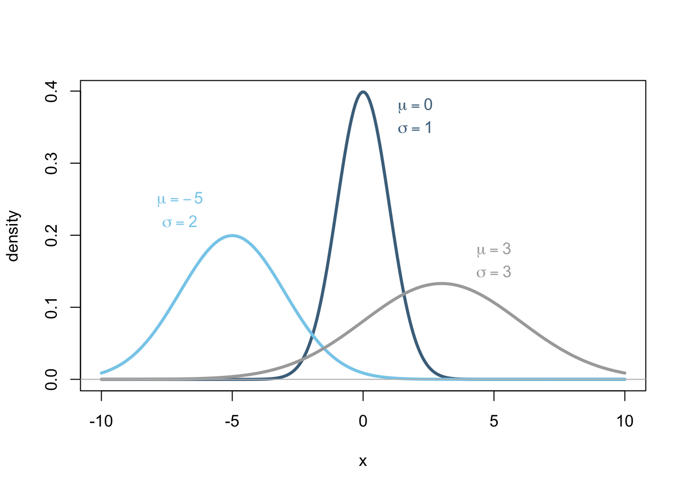
The usefulness of the normal distribution is that we know which values of data are likely and which are unlikely by just knowing three things:
that the data is normally distributed,
\(\mu\), the mean of the distribution, and
\(\sigma\), the standard deviation of the distribution.
For example, as shown in the plot above, a value of \(x=-8\) would be very probable for the normal distribution with \(\mu=-5\) and \(\sigma=2\) (light blue curve). However, the value of \(x=-8\) would be very unlikely to occur in the normal distribution with \(\mu=3\) and \(\sigma=3\) (gray curve). In fact, \(x=-8\) would be even more unlikely an occurance for the \(\mu=0\) and \(\sigma=1\) distribution (dark blue curve).