Chapter 2 Introduction to the Normal Distribution and Z-Scores

2.1 The Normal Distribution

2.1.1 Intro

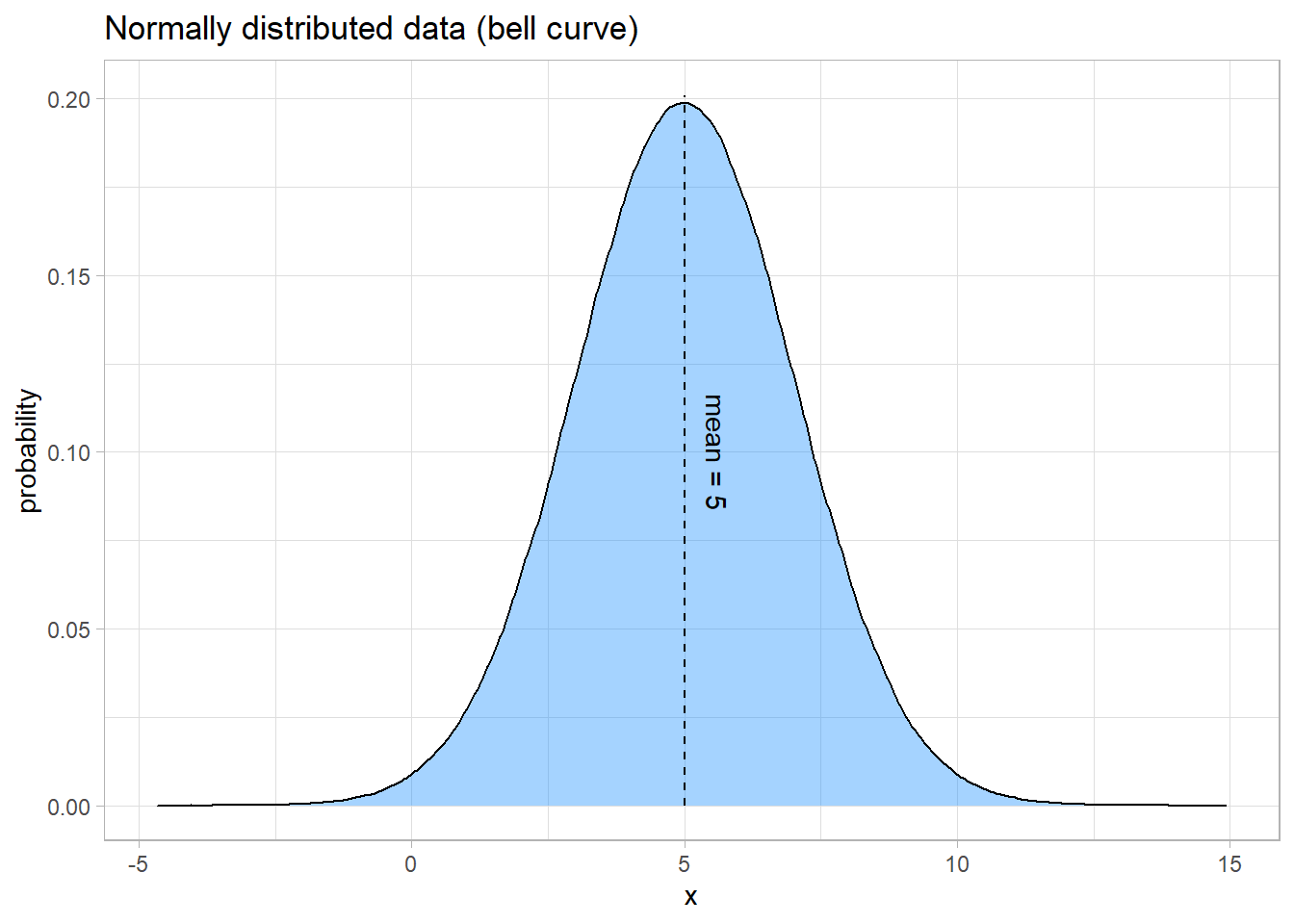
There are many different ways that data can be distributed, but the most important and statistically powerful type of distribution is the normal distribution. While you may not be familiar with its properties, you’re likely familiar with the distribution itself. The main idea is that there is some central value (the mean) that is the most probable value in the data. On either side of the mean, the probability of the data decreases symmetrically. The spread of the data can be described by the standard deviation (or the variance). The higher the standard deviation, the more spread out the data is.

Here is an example of a normal curve:

2.1.2 Example - Batting Averages

As it turns out, normal distributions show up naturally all over the place. One example is the distribution of batting averages in baseball.

Source: MATH 221 Textbook

In baseball, a player called the “pitcher” throws a ball to a player called the “batter.” The batter swings a wooden or metal bat and tries to hit the ball. A “hit” is made when the batter successfully hits the ball and runs to a point in the field called first base. A player’s batting average is calculated as the ratio of the number of hits a player makes divided by the number of times the player has attempted to hit the ball or in other words, been “at bat.” Sean Lahman reported the batting averages of several professional baseball players in the United States. (Lahman, 2010) The file BattingAverages.xlsx contains his data.

The following histogram summarizes the batting averages for these professional baseball players:

Notice the bell-shaped distribution of the data.

Suppose we want to estimate the probability that a randomly selected player will have a batting average that is greater than 0.280. One way to do this would be to find the proportion of players in the data set who have a batting average above 0.280. We can do this by finding the number of players who fall into each of the red-colored bins below and dividing this number by the total number of players.

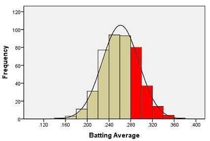
In other words, we could find the proportion of the total area of the bars that is shaded red out of the combined area of all the bars. This gives us the proportion of players whose batting averages are greater than 0.280.

Out of the 446 players listed, there are a total of 133 players with batting averages over 0.280. This suggests that the proportion of players whose batting average exceeds 0.280 is:

\[\displaystyle{\frac{133}{446}} = 0.298\]

Alternatively, we can use the fact that the data follow a bell-shaped distribution to find the probability that a player has a batting average above 0.280.

2.1.3 Density Curves

The bell-shaped curve superimposed on the histogram above is called a density curve. It is essentially a smooth histogram. Notice how closely this curve follows the observed data.

The density curve illustrated on the histogram of the batting average data is special. It is called a normal density curve. This density curve is symmetric and has a bell-shape.

The normal density curve is also referred to as a normal distribution or a “Gaussian” distribution (after Carl Friedrich Gauss.)

The normal density curve appears in many applications in business, nature, medicine, psychology, sociology, and more. We will use the normal density curve extensively in this course.

All density curves, including normal density curves, have two basic properties:

The total area under the curve equals 1.
The density curve always lies on or above the horizontal axis.

Because of these two properties, the area under the curve can be treated as a probability. If we want to find the probability that a randomly selected baseball player will have a batting average between some range of values, we only need to find the area under the curve in that range. This is illustrated by the region shaded in blue in the figure below.

Again, normal density curve is uniquely determined by its mean, \(\mu\), and its standard deviation, \(\sigma\). So, if random variables follow a normal distribution with a known mean and standard deviation, then we can calculate any probabilities related to that variable by finding the area under the curve.

When the mean of a normal distribution is 0 and its standard deviation is 1, we call it the standard normal distribution, an important concept which we’ll cover later in the chapter.

2.2 Z-Scores

Source: MATH 221 Textbook

2.2.1 Introduction to Z-scores

In Ghana, the mean height of young adult women is normally distributed with mean \(159.0\) cm and standard deviation \(4.9\) cm. (Monden & Smits, 2009) Serwa, a female BYU-Idaho student from Ghana, is \(169.0\) cm tall. Her height is \(169.0 - 159.0 = 10\) cm greater than the mean. When compared to the standard deviation, she is about two standard deviations (\(\approx 2 \times 4.9\) cm) taller than the mean.

The heights of men are also normally distributed. The mean height of young adult men in Brazil is \(173.0\) cm (“Oramento,” 2010), and the standard deviation for the population is \(6.3\) cm. (Castilho & Lahr, 2001) A Brazilian BYU-Idaho student, Gustavo, is \(182.5\) cm tall. Compared to other Brazilians, he is taller than the mean height of Brazilian men.

When we examined the heights of Serwa and Gustavo, we compared their height to the standard deviation. If we look carefully at the steps we did, we subtracted each individual’s height from the mean height for people of the same gender and nationality.

2.2.2 Computing Z-scores

This shows how much taller or shorter the person is than the mean height. In order to compare the height difference to the standard deviation, we divide the difference by the standard deviation. This gives the number of standard deviations the individual is above or below the mean.

For example, Serwa’s height is 169.0 cm. If we subtract the mean and divide by the standard deviation, we get \[z = \frac{169.0 - 159.0}{4.9} = 2.041\] We call this number a \(z\)-score. The \(z\)-score for a data value tells how many standard deviations away from the mean the observation lies. If the \(z\)-score is positive, then the observed value lies above the mean. A negative \(z\)-score implies that the value was below the mean.

We compute the \(z\)-score for Gustavo’s height similarly, and obtain \[z = \frac{182.5 - 173.0}{6.3} = 1.508\] Gustavo’s \(z\)-score is 1.508. As noted above, this is about one-and-a-half standard deviations above the mean. In general, if an observation \(x\) is taken from a random process with mean \(\mu\) and standard deviation \(\sigma\), then the \(z\)-score is \[z = \frac{x -\mu }{\sigma}\]

The \(z\)-score can be computed for data from any distribution, but it is most commonly applied to normally distributed data.

2.3 Standard Normal Distributions

Source: MATH 221 Textbook (excluding graphic)

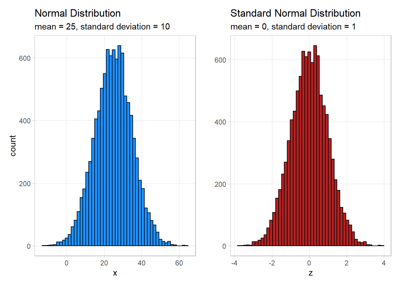
A standard normal distribution is a normal distribution with a mean of 0 and a standard deviation of 1. We call it a standard normal because the values are standardized. No matter what the distribution is about (heights, temperatures, etc.), if the distribution is a standard normal then they are all on the same scale. This is useful when comparing distributions because differences in units or scales no longer need to be considered in the comparison.

As shown below, standardizing values doesn’t alter the shape of the distribution. The counts in each bin change very little, and any discrepancies are likely to be as a result of rounding error as much as anything.

## `summarise()` ungrouping output (override with `.groups` argument)

variable	mean	standard deviation
x	24.98	9.98
z	0	1

2.4 Rules of Thumb

2.4.1 68-95-99.7% Rule

Source: MATH 221 Textbook

Heights of women (or men) in a particular population follow a normal distribution. Knowing this, think about the following statement:

Most people’s heights are close to the mean. A few are very tall or very short.

While this may be true, suppose we would like to make a more precise statement than this. To do so, we can use the following rule of thumb:

For any bell-shaped distribution:
- 68% of the data will lie within 1 standard deviation of the mean,
- 95% of the data will lie within 2 standard deviations of the mean, and
- 99.7% of the data will lie within 3 standard deviations of the mean.

68-95-99.7% Rule

This is called the 68-95-99.7% Rule for Bell-shaped Distributions. Some statistics books refer to this as the Empirical Rule.

Approximately 68% of the observations from a bell-shaped distribution will be between the values of \(\mu -~\sigma~\) and \(\mu +~\sigma~\). Consider the heights of young adult women in Ghana. We expect that about 68% of Ghanian women have a height between the values of \[\mu -~\sigma = 159.0 - 4.9 = 154.1~\text{cm}\] and \[\mu +~\sigma = 159.0 + 4.9 = 163.9~\text{cm}.\]

So, if a female is chosen at random from all the young adult women in Ghana, about 68% of those chosen will have a height between 154.1 and 163.9 cm. Similarly, 95% of the women’s heights will be between the values of \[\mu - 2\sigma = 159.0 - 2(4.9) = 149.2~\text{cm}\] and \[\mu + 2\sigma = 159.0 + 2(4.9) = 168.8~\text{cm}.\]

Finally, 99.7% of the women’s heights will be between \[\mu - 3\sigma = 159.0 - 3(4.9) = 144.3~\text{cm}\] and \[\mu + 3\sigma = 159.0 + 3(4.9) = 173.7~\text{cm}.\]

Consider again the plots from above, this time with 1, 2, and 3 standard deviations from the mean marked.

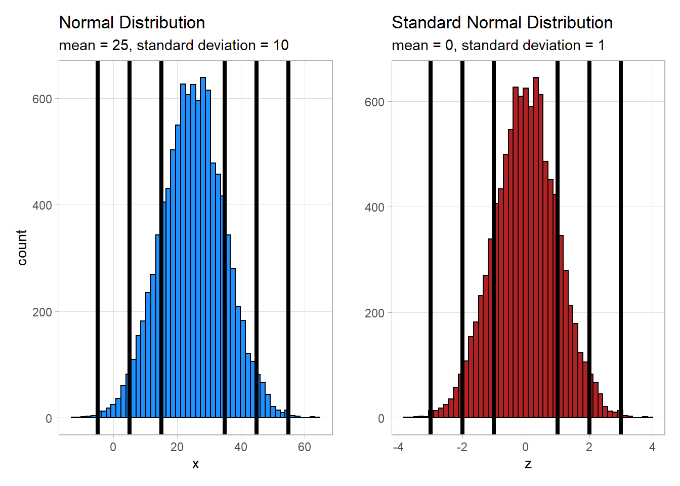
As you can see, the spread of the data is the same whether the data has been standardized or not. The 68-95-99.7% Rule still holds true because even though the scale has changed the relative distance of the data from the mean has not.

Unusual Events

If a \(z\)-score is extreme (either a large positive number or a large negative number), then that suggests that that observed value is very far from the mean. The 68-95-99.7% rule states that 95% of the observed data values will be within two standard deviations of the mean. This means that 5% of the observations will be more than 2 standard deviations away from the mean (either to the left or to the right).

We define an unusual observation to be something that happens less than 5% of the time. For normally distributed data, we determine if an observation is unusual based on its \(z\)-score. We call an observation unusual if \(z < -2\) or if \(z > 2\). In other words, we will call an event unusual if the absolute value of its \(z\)-score is greater than 2.

2.4.2 Standard Deviation Estimation

While the concept of the standard deviation isn’t terribly complicated, computing it by hand isn’t particularly convenient. A general rule of thumb for estimating it is to subtract the minimumum from the maximum, and then divide that difference by either 4 or 6.

\[ \frac{Maximum - Minimum} {\text{4 or 6} } \]

If accuracy is important, it is recommended that you actually compute the standard deviation using software or the formula here.

See this website for a more detailed explanation on why this trick is a valid method, but it follows the principle that nearly all of the data should fall within 2 (or 3) standard deviations on either side of the mean, or within 4 (or 6) total standard deviations.

References

Lahman, S.Sean lahman’s baseball archive. Retrieved November, 2010, from http://www.baseball1.com/