Medical Wire DOE
Answer Key
Assignment Description
This answer key provides the process (and results) that I would go through to address the question of significant effects based on a designed experiment. You can right click and download the Rmd file to see this whole answer key which will allow your final to look similar. An important part is in the YAML or stuff between the dashed lines at the top of the Rmd file. By using what I have you can hide code, so that the paper flows well and your code can still be checked. Remember that your finals are to be submitted as an html document. An example of this header information is shown below.
---
title: "Medical Wire DOE"
author: "Answer Key"
output:
  html_document:
    toc: true
    code_folding: hide
---
Grading of the final
- Format will be part of the grade (so follow the flow of this example). When presenting information to a client it is important that the message flows and that the results are concise. The flow and feel should be similar to a memo within a company.
- Narrative will be part of the grade. Do the final like you are writing up a project for your boss.
- Correct answers will be part of the grade.
- Your ability to explain your answers and document your ideas will be a big part of your grade. Your data and conclusions about interactions and significance will be different from mine. Use your own wording.
- Don’t copy from others in the class. You can use the internet, Kris, and I as much as you want in completing the exam.
Medical Wire Design of Expirement
Our data set of the Medical wire material has three factors with each at a high/low level. The factors are
- Drawing Machine
- Die Reduction Angle
- Die Bearing Length
We need to identify which factors and their interactions are significant. Before we begin analysis with statistical methods let’s look at a plot of the data. Note that during the analysis that a value of “0” means low and a value of “1” means high for each respective factor.
wire_example = read.csv(file="http://byuistats.github.io/M330/data/wire.csv")
wire_example_wide = read.csv(file = "http://byuistats.github.io/M330/data/wire_wide.csv")

# Now we need to make the variables factors
wire_example$Drawing_Machine = as.factor(wire_example$Drawing_Machine)
wire_example$Die_Reduction_Angle = as.factor(wire_example$Die_Reduction_Angle)
wire_example$Die_Bearing_Length = as.factor(wire_example$Die_Bearing_Length)


### Plot our Data

# First calculate means
wire.cellmeans = ddply(.data=wire_example,.variables = .(Drawing_Machine,Die_Reduction_Angle,Die_Bearing_Length),.fun=function(x){
  data.frame(strength=mean(x$strength))
} )

wire.grandmean = mean(wire_example$strength)

wire.dmmeans = ddply(.data=wire_example,.variables = .(Drawing_Machine),.fun=function(x){
  data.frame(strength=mean(x$strength))
} )
Data Visualization
From the plot below we can see that there may be an interaction between Drawing Machine and Die Bearing Length that is significant. Namely, that the high levels of each factor improve the wire properties. Finally, it looks like the low level of Die Reduction Angle may be significant as well. At this point, the graph does not clearly justify these conclusions but hints at what may be significant in the analysis to follow.
wire_plot = ggplot(data=wire_example,aes(x=Die_Reduction_Angle,y=strength))+
  geom_boxplot()+
  geom_jitter(height=0,width=.25)+
  theme_bw()+labs(y="Quality:low number good (YS/UTS)")

wire_plot +
  facet_wrap(~Drawing_Machine+Die_Bearing_Length,labeller = "label_both",nrow=1)+
  geom_hline(yintercept=wire.grandmean,size=1.5,colour="blue",alpha=.5)+
  geom_point(data=wire.cellmeans,size=4,col="darkgrey",shape=15,alpha=.75)+
  geom_point(data=wire.cellmeans,size=2,col="black",shape=15,alpha=.75)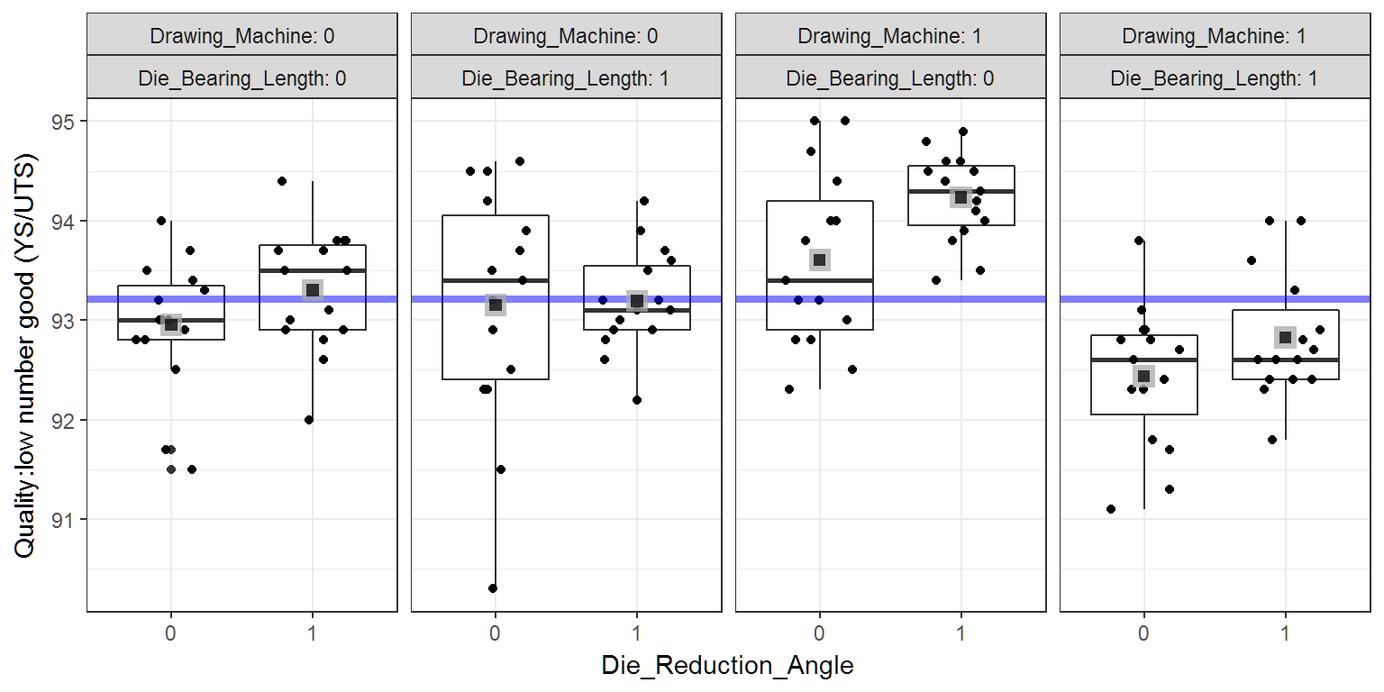
First we will fit the full model with all the 2-way and 3-way interactions so that we can check our assumptions of equal variance and normality as they relate to ANOVA results.
wire.aov.all=aov(strength~Drawing_Machine*Die_Reduction_Angle*Die_Bearing_Length,data=wire_example)Constant Variance Check
From the table and plot below, we see that our constant variance assumption is rejected for Die Reduction Angle and is suspect for the 3-way interaction. While we failed the constant variance assumption, we have equal sample sizes in each group and we know that, “ANOVA is also fairly robust to [departures from] the equal variances assumption, provided the samples are about the same size for all groups.” [1]. So we will move forward with the ANOVA analysis.
# Now check assumptions
equal.variance = anova(aov(resid(wire.aov.all)^2~Drawing_Machine*Die_Reduction_Angle*Die_Bearing_Length,
             data=wire_example))
datatable(equal.variance)%>%formatRound(columns=1:5, digits=2)
plot(wire.aov.all,which=1)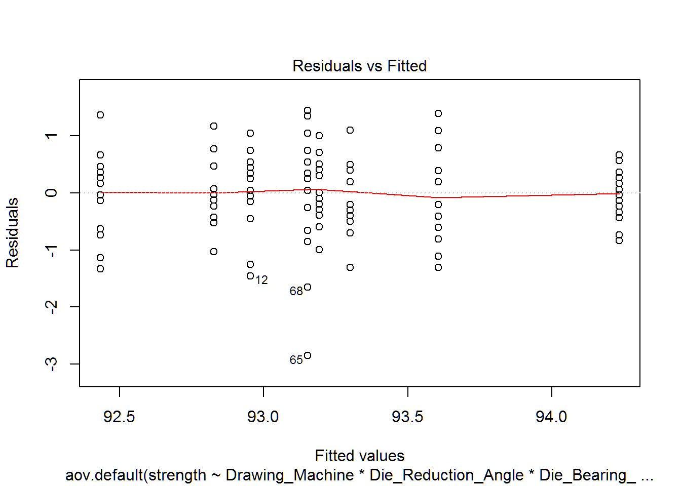
Normality Check
Our Normal probability plot and the resulting Shapiro-Wilk test hint that our residuals might not be normally distributed. From our previous reference we read, “ANOVA is robust to the normality assumption-it can handle”kinda sorta" normal data-if your sample sizes are large enough.“[1]
Our samples sizes are not really big (15 observations per group), but our departures from normality are not too strong either. As both assumptions are not fully met, our resulting p-values will be a little incorrect, but should be sufficient for us to identify significant differences in the mean effects
# Normality of residuals
norm.test = shapiro.test(resid(wire.aov.all))
norm.test
##
## Shapiro-Wilk normality test
##
## data: resid(wire.aov.all)
## W = 0.97697, p-value = 0.03727plot(wire.aov.all,which=2)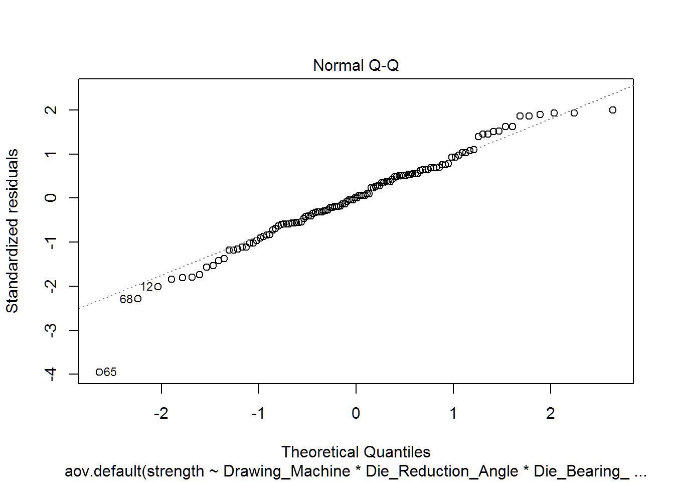
Effect Significance Analyses
From the table below we see that the 3-way interaction is not significant and we can remove it from our model.
wire.aov.all=aov(strength~Drawing_Machine+Die_Reduction_Angle+Die_Bearing_Length+
                          Drawing_Machine:Die_Reduction_Angle+Drawing_Machine:Die_Bearing_Length+
                          Die_Reduction_Angle:Die_Bearing_Length+
                          Drawing_Machine:Die_Reduction_Angle:Die_Bearing_Length,data=wire_example)

datatable(anova(wire.aov.all))%>%formatRound(columns=1:5, digits=2)
Without the 3-way interaction being modeled, we can evaluate which 2-way interactions are significant with the table below. The interaction of Drawing Machine and Die Bearing Length is significant so we will keep it in the model. All other 2-way interactions will be removed from the model.
# looks like there isn't.  Let's remove and check two way
# see page 403 for code example and description
wire.aov.n3way=aov(strength~Drawing_Machine*Die_Reduction_Angle+ Drawing_Machine*Die_Bearing_Length+Die_Bearing_Length*Die_Reduction_Angle,data=wire_example)
datatable(anova(wire.aov.n3way))%>%formatRound(columns=1:5, digits=2)
#one significant two way interactionEffect Size Conclusions
This ANOVA table below is our final model that we will use to draw conclusions about our experiment. Note that Drawing Machine alone is not a significant effect, but that it’s interaction with Die Bearing Length necessitates keeping it in the final model.
wire.aov.signif=aov(strength~Drawing_Machine+Die_Bearing_Length+Die_Reduction_Angle+Drawing_Machine:Die_Bearing_Length,data=wire_example)

datatable(anova(wire.aov.signif))%>%formatRound(columns=1:5, digits=2)
#TukeyHSD(wire.aov.signif)
#plot(TukeyHSD(wire.aov.signif))
# We can also get them out a different way
wire.ls = lsmeans(wire.aov.signif,~Drawing_Machine+Die_Reduction_Angle+Die_Bearing_Length+Drawing_Machine:Die_Bearing_Length)
drawing.ls = lsmeans(wire.aov.signif,~Drawing_Machine)
DRA.ls = lsmeans(wire.aov.signif,~Die_Reduction_Angle)
DBL.ls = lsmeans(wire.aov.signif,~Die_Bearing_Length)
drawing_DBL.ls = lsmeans(wire.aov.signif,~Drawing_Machine:Die_Bearing_Length)We know that Die Reduction Angle and Die Bearing Length are significant main effects. Also, from our ANOVA model we know that the interaction effect between Drawing Machine and Die Bearing Length is significant as well. The estimates of the size of these significant effects are shown below.
Effects Estimates
The Die Reduction Angle has a .35 improvement in the wire quality measure at the low level.
effect.DRA = summary(pairs(DRA.ls))
#effect.DRA$contrast = as.character(effect.DRA$contrast)
datatable(effect.DRA)%>%formatRound(columns=2:6, digits=2)
The Die Bearing Length has a .62 improvement in the wire quality measure at the high level.
effect.DBL = summary(pairs(DBL.ls))
datatable(effect.DBL)%>%formatRound(columns=2:6, digits=2)
This effects table below shows six possible interaction variations between Drawing Machine and Die Bearing Length. From this table we see that having each of the two factors at their low level as compared to having the Drawing Machine high and Die Bearing Length low results in the largest effect of 1.29 improvement.
effect.interaction = summary(pairs(drawing_DBL.ls))
datatable(effect.interaction)%>%formatRound(columns=2:6, digits=2)
Conclusions
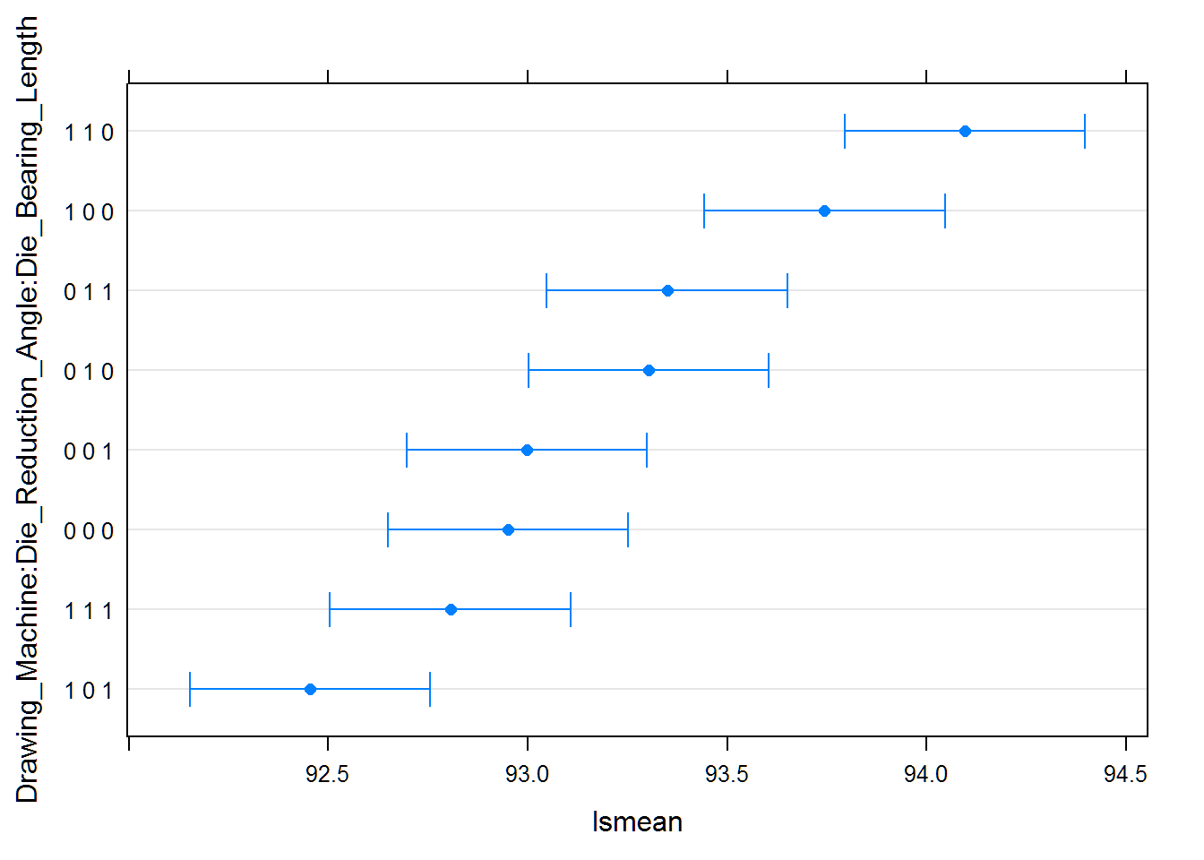
From the table and plot below, we formalize the same conclusions that were hinted by the original plot above. We see that there is a significant interaction between Drawing Machine and Die Bearing Length. Specifically, that the high levels of each factor improve the wire properties. Finally, the low level of Die Reduction Angle should be used as it was a significant factor as well.
With these results we can expect to our wire properties to be 92.45 (YS/UTS). With 95% confidence, our wire properties will be between 92.15 and 92.76 (YS/UTS).
datatable(cld(wire.ls))%>%formatRound(columns=4:8, digits=2)plot(cld(wire.ls))