Code Notes on Section 1.5 Akritas
Reading data from Akritas datasets
An R script with the same basic information can be found here
New Functions
I am introducing new R functions to what Akritas has given you up to this point.
- file.path()
- with()
- head()
- tail()
- str()
- summary()
Remember that in R you can type ?file.path and ?with to see what the functions do in more detail.
Using file.path() and a data.dir object
If you have a local download location, type in the folder of the location where you extracted the data.
data.dir = "c://m330data"Or you can pull it directly from the website listed in the book each time.
data.dir = "http://media.pearsoncmg.com/cmg/pmmg_mml_shared/mathstatsresources/Akritas"With data.dir defined you can use the following command to read in the data
br = read.table(file.path(data.dir,"BearsData.txt"),header=T)Alternatives to attach()
The attach command has some benefit and I used it a little when I was a student. However, I have since stopped using it as I think it can create problems (which we can discuss later if you want). For example, I would tweak the code from page 20 to the following code
lv = read.table(file.path(data.dir,"MarketShareLightVeh.txt"),header=T)
pie(lv$Percent,labels=lv$Company,col=rainbow(length(lv$Percent)))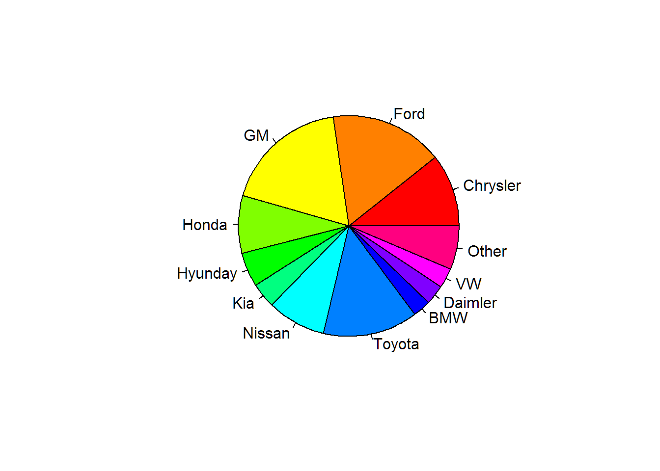
Another options is to use the with() command. The attach() command alters the entire R session while the with() only alters the reference space for the specific function
with(lv,pie(Percent,labels=Company,col=rainbow(length(Percent))))
Hathaway Data Dos
I like to do a few things to make sure the data is read in correctly. It involves using the head/tail commands. These commands let us see the first few rows of data and the column and row names.
head(br) ## ID Sex Age Head.L Head.W Neck.G Chest.G Weight
## 1 41 F 23 12.5 5.0 20.5 38.0 142
## 2 48 M 81 15.5 8.0 31.0 54.0 416
## 3 69 M * 16.0 8.0 32.0 52.0 432
## 4 83 M 117 15.5 7.5 32.0 54.5 476
## 5 238 M 70 15.0 6.5 28.0 45.0 334
## 6 274 F 57 13.5 7.0 20.0 38.0 204tail(br)## ID Sex Age Head.L Head.W Neck.G Chest.G Weight
## 45 665 M * 13.0 6.5 20.5 36.5 154
## 46 670 M * 16.0 7.5 28.0 45.0 316
## 47 673 F * 13.5 5.5 19.5 35.0 158
## 48 675 F * 12.5 5.5 19.0 32.0 120
## 49 679 M * 15.5 7.5 25.5 43.0 324
## 50 681 M * 14.5 7.0 22.0 38.0 196The str() command shows the columns in a different format and also provides the characteristics of the columns. Notice the description of each variable as int, Factor, or num. Other types are character and logical.
str(br)## 'data.frame': 50 obs. of 8 variables:
## $ ID : int 41 48 69 83 238 274 518 520 522 525 ...
## $ Sex : Factor w/ 2 levels "F","M": 1 2 2 2 2 1 2 1 2 2 ...
## $ Age : Factor w/ 18 levels "*","10","11",..: 7 15 1 4 14 12 11 18 6 5 ...
## $ Head.L : num 12.5 15.5 16 15.5 15 13.5 13.5 9 13 16 ...
## $ Head.W : num 5 8 8 7.5 6.5 7 7 4.5 6 9.5 ...
## $ Neck.G : num 20.5 31 32 32 28 20 24 12 19 30 ...
## $ Chest.G: num 38 54 52 54.5 45 38 39 19 30 48 ...
## $ Weight : int 142 416 432 476 334 204 204 26 120 436 ...The summary() function provides an overall summary of each column based on their respective characteristics.
summary(br)## ID Sex Age Head.L Head.W
## Min. : 41.0 F:15 * :15 Min. : 9.00 Min. :4.00
## 1st Qu.:531.5 M:35 10 : 3 1st Qu.:12.62 1st Qu.:5.50
## Median :558.5 21 : 3 Median :13.50 Median :6.50
## Mean :528.9 34 : 3 Mean :13.43 Mean :6.24
## 3rd Qu.:619.0 45 : 3 3rd Qu.:14.50 3rd Qu.:7.00
## Max. :681.0 57 : 3 Max. :17.00 Max. :9.50
## (Other):20
## Neck.G Chest.G Weight
## Min. :12.00 Min. :19.00 Min. : 26.0
## 1st Qu.:19.00 1st Qu.:32.00 1st Qu.:121.2
## Median :21.00 Median :36.75 Median :161.0
## Mean :21.92 Mean :37.65 Mean :202.8
## 3rd Qu.:25.88 3rd Qu.:44.00 3rd Qu.:276.0
## Max. :32.00 Max. :55.00 Max. :476.0
##