8.4 Decision Errors
A simulation Game
Today we are going to play a little simulation game. In this simulation we are going to create two different distributions. Let’s say we know following advertised truth about the number of miles of our company’s brand of tires will last(1):
Ho : μ = 60k
If we are the company that sells these tires…
- How many miles above 60k in this truth would matter to us?
- Would a 1k mile improvement matter?
- Would a 10k mile improvement matter?
Let’s say that we cared about an improvement of 3k and that we know the tread life has a σ = 12k. Then
Ha : μ = 63k
nsize = 36
sd_value = 12
diff = 3
null_mean = 60

## using a known sd power calculation
null_distribution = rnorm(n=nsize,mean=null_mean,sd=sd_value)
alt_distribution = rnorm(n=nsize,mean=null_mean+diff,sd=sd_value)
p95 = qnorm(.95,mean=null_mean,sd=sd_value/sqrt(nsize))
qnorm(.1,mean=null_mean+diff,sd=sd_value/sqrt(nsize))
## [1] 60.4369typeII = pnorm(p95,mean=null_mean+diff,sd=sd_value/sqrt(nsize))
1-typeII## [1] 0.4424132repeats_a = replicate(500,mean(rnorm(n=nsize,mean=null_mean+diff,sd=sd_value)))
repeats_o = replicate(500,mean(rnorm(n=nsize,mean=null_mean,sd=sd_value)))
sum(repeats_a>p95)/500## [1] 0.46sum(repeats_o>p95)/500## [1] 0.058pdata = data.frame(values=c(repeats_o,repeats_a),hypothesis= rep(c("Ho","Ha"),each=500))
# ggplot(data=pdata,aes(x=hypothesis,y=values))+
# geom_boxplot()
#
# ggplot(data=pdata,aes(x=values))+
# geom_histogram(colour="white")+
# facet_wrap(~hypothesis,ncol=1)The above example was using a known standard deviation, σ, let’s realize that the tire company does not know their true standard deviation. From previous small scale studies they believe the standard deviation to be be 8k. They would like you to tell them how many customers they will need to track to be able to validate that their tires do in fact last 60k miles on average. If their tires do last 63k miles on average then they want to be able to advertise the added mileage. So they want to be able to distinguish an alternative hypothesis of 63k miles.
Your Job
This guy actually tracked his own tires. We don’t have time to do this, but I am sure car dealers have a way to test this. Or maybe they don’t
- Help the tire company know how many customers they should sample to show that their tires do you in fact last 60k miles on average if they want to be able to tell a difference between an average of 60k and 63k?
- you need to write a sentence that tells them what power they should use.
- you need to show them a plot of trade-off between the sample size and resulting power.
make a plot like the previous that shows power to detect a difference of 6k.
library(pwr)## Warning: package 'pwr' was built under R version 3.3.2# d = effect size, effect size is the difference divided by the sd.
pwr.t.test(n=36,3/12,.05,power=NULL,"one.sample","greater")##
## One-sample t test power calculation
##
## n = 36
## d = 0.25
## sig.level = 0.05
## power = 0.4309684
## alternative = greater# there is also a similar function in R
# power.t.testSome notes on Type II error and Confidence
We could allow ourselves to make Type I decision errors in both directions. Then the area in the middle is the area that would describe the compliment of a Type I decision error or the confidence. So if we set Type I error to α = .05, then we will be 95% (100 × (1 − α)) confident that the true mean is is within our interval. The picture below depicts this for a normal distribution.
normTail(,M=c(-1.96,1.96))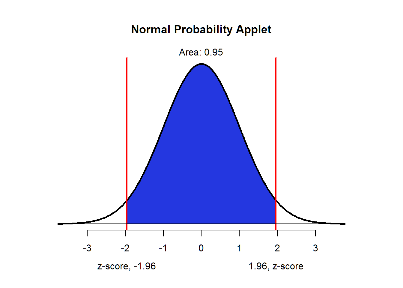
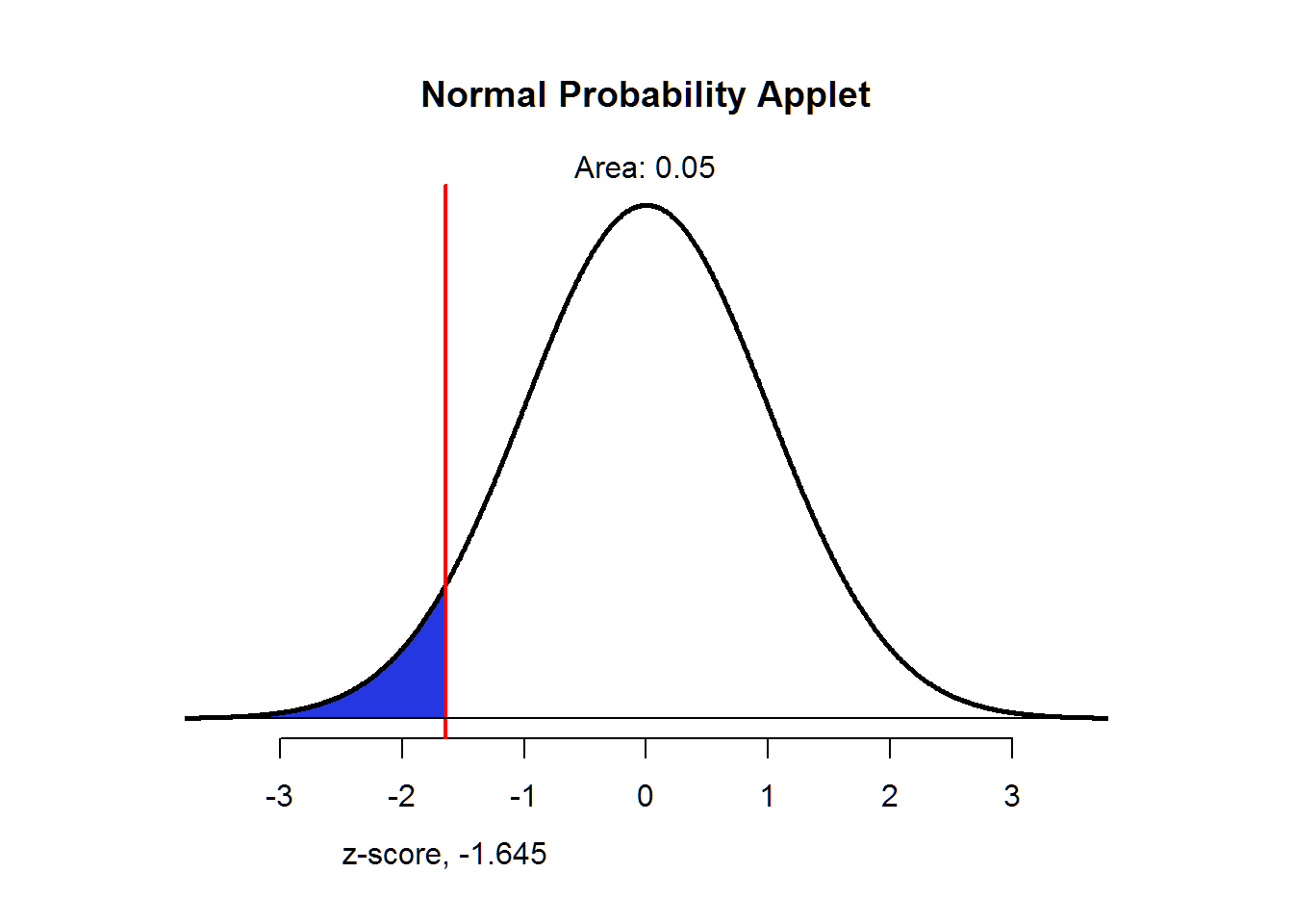
However, we don’t have to allow for decision errors in both directions. We could have a one-sided confidence interval which is generally called an upper-confidence level (UCL) or a lower-confidence level (LCL). In the one-sided case, we would have the same confidence (100 × (1 − α)). However, we would put all of our Type I risk in one tail. The next plot shows α instead of confidence.
normTail(,L=c(-1.645))