Class Example (6.2)
Getting Estimates from Data
Akritas’ remarks are generally very insightfull. Please read remark 6.2-1. Let’s do some examples below. Copy the code snippets below. Or you can download this webpage as an Rmd file.
Uniform Test Case
In his remark, he says the model based estimators are better if the correct model is known. However, model based estimates can be misleading (read horribly wrong) if the model assumption is incorrect.
Code
library(reshape)
library(ggplot2)
uniform_runs = function(sample=30){
  unif_data = runif(sample)
  model_mean = (max(unif_data)-min(unif_data))/2
  free_mean = mean(unif_data)
  c("model"=model_mean,"free"=free_mean)
}

wide_estimates = replicate(1700,uniform_runs(sample=115))
apply(wide_estimates,1,mean)
apply(wide_estimates,1,sd)

long_estimates = melt(wide_estimates)

qplot(data=long_estimates,x=value)+facet_wrap(~X1,ncol=1,scales="free_y")
Evaluated Code
library(reshape)
library(ggplot2)
uniform_runs = function(sample=30){
  unif_data = runif(sample)
  model_mean = (max(unif_data)-min(unif_data))/2
  free_mean = mean(unif_data)
  c("model"=model_mean,"free"=free_mean)
}

wide_estimates = replicate(1700,uniform_runs(sample=115))
apply(wide_estimates,1,mean)
## model free
## 0.4915459 0.5006877apply(wide_estimates,1,sd)## model free
## 0.005867268 0.026887230long_estimates = melt(wide_estimates)
qplot(data=long_estimates,x=value)+facet_wrap(~X1,ncol=1,scales="free_y")## `stat_bin()` using `bins = 30`. Pick better value with `binwidth`.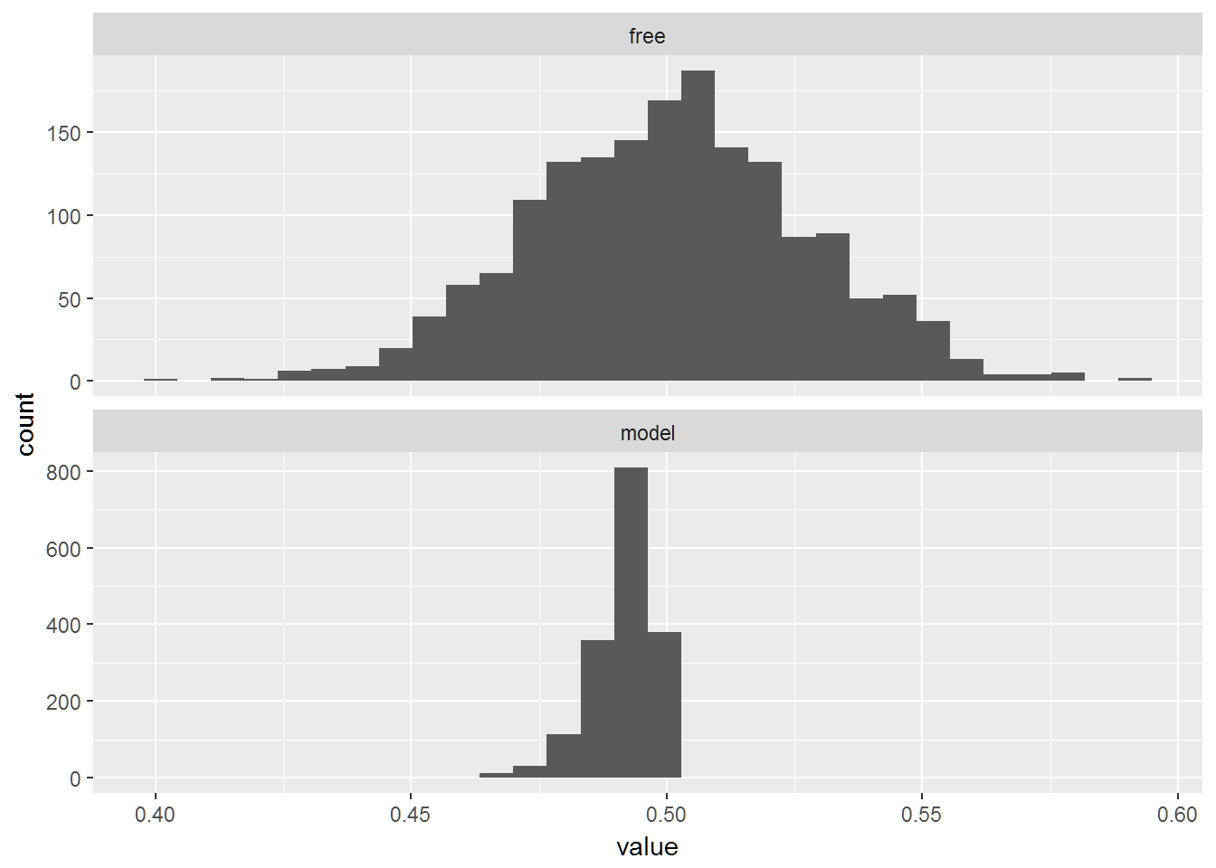
Now what happens if we use a uniform model to estimate the mean when in fact it is not uniform (it is normal).
Code
library(reshape)
library(ggplot2)
normal_runs = function(sample=15){
  unif_data = rnorm(sample)
  model_mean = (max(unif_data)-min(unif_data))/2
  free_mean = mean(unif_data)
  c("model"=model_mean,"free"=free_mean)
}

wide_estimates_bad = replicate(1700,normal_runs(sample=115))
apply(wide_estimates_bad,1,mean)
apply(wide_estimates_bad,1,sd)

long_estimates_bad = melt(wide_estimates_bad)

qplot(data=long_estimates_bad,x=value)+facet_wrap(~X1,ncol=1,scales="free_y")
Evaluated Code
library(reshape)
library(ggplot2)
normal_runs = function(sample=15){
  unif_data = rnorm(sample)
  model_mean = (max(unif_data)-min(unif_data))/2
  free_mean = mean(unif_data)
  c("model"=model_mean,"free"=free_mean)
}

wide_estimates_bad = replicate(1700,normal_runs(sample=115))
apply(wide_estimates_bad,1,mean)
## model free
## 2.556818354 0.001176282apply(wide_estimates_bad,1,sd)## model free
## 0.29206107 0.09146539long_estimates_bad = melt(wide_estimates_bad)
qplot(data=long_estimates_bad,x=value)+facet_wrap(~X1,ncol=1,scales="free_y")## `stat_bin()` using `bins = 30`. Pick better value with `binwidth`.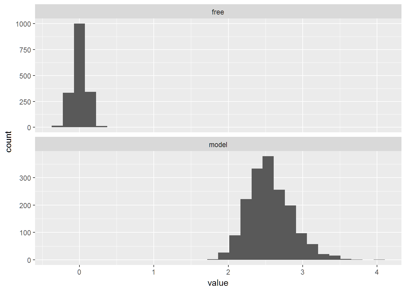
Wiebull Example
Here is a nice cheat sheet for the Weibull Distribution. We are also going to use the MASS library to help us fit a model to our data. Don’t worry about understanding the fitting procedure (6.3.2 Describes the method we are using with the fitdsitr function).
We are going to generate random data from a known distribution Weibull and then see how well our estimates represents the truth.
Code
library(MASS)
n=10
percentile_desired = .01
shape_w = 30
scale_w = 60

X5 = rweibull(n,shape_w,scale_w)

fit_w = fitdistr(X5,"weibull")
fit_n = fitdistr(X5,"normal")
fit_n
mean(X5); sd(X5)

hist(X5)
qqnorm(X5)
qqline(X5)

# The upper percentile
# Model Free
quantile(X5,1-percentile_desired)
# Model Based: Not correct Model
qnorm(1-percentile_desired,mean=fit_n$estimate["mean"],sd=fit_n$estimate["sd"])
# Model Based: Correct Distribution, Estimated Parameters
qweibull(1-percentile_desired,shape=fit_w$estimate["shape"],scale=fit_w$estimate["scale"])
# Model Based: Correct Distribution, Correct Parameters
qweibull(1-percentile_desired,shape_w,scale_w)

# Now look at the lower percentile
# Model Free
quantile(X5,percentile_desired)
# Model Based: Not correct Model
qnorm(percentile_desired,mean=fit_n$estimate["mean"],sd=fit_n$estimate["sd"])
# Model Based: Correct Distribution, Estimated Parameters
qweibull(percentile_desired,shape=fit_w$estimate["shape"],scale=fit_w$estimate["scale"])
# Model Based: Correct Distribution, Correct Parameters
qweibull(percentile_desired,shape_w,scale_w)
Evaluated Code
library(MASS)
n=10
percentile_desired = .01
shape_w = 30
scale_w = 60

X5 = rweibull(n,shape_w,scale_w)

fit_w = fitdistr(X5,"weibull")
fit_n = fitdistr(X5,"normal")
fit_n
## mean sd
## 56.6151645 3.4152786
## ( 1.0800059) ( 0.7636795)mean(X5); sd(X5)## [1] 56.61516## [1] 3.60002hist(X5)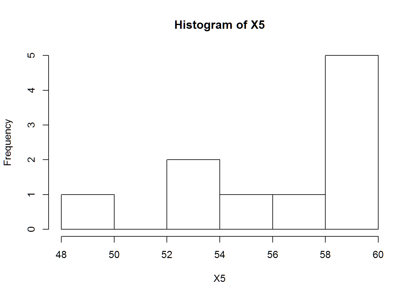
qqnorm(X5)
qqline(X5)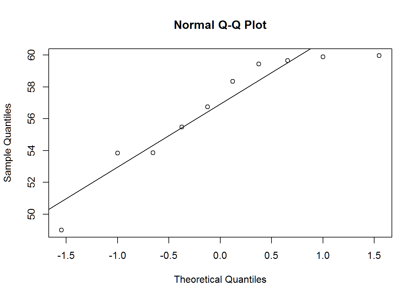
# The upper percentile
# Model Free
quantile(X5,1-percentile_desired)
## 99%
## 59.94553# Model Based: Not correct Model
qnorm(1-percentile_desired,mean=fit_n$estimate["mean"],sd=fit_n$estimate["sd"])## [1] 64.56029# Model Based: Correct Distribution, Estimated Parameters
qweibull(1-percentile_desired,shape=fit_w$estimate["shape"],scale=fit_w$estimate["scale"])## [1] 62.08192# Model Based: Correct Distribution, Correct Parameters
qweibull(1-percentile_desired,shape_w,scale_w)## [1] 63.13344# Now look at the lower percentile
# Model Free
quantile(X5,percentile_desired)## 1%
## 49.435# Model Based: Not correct Model
qnorm(percentile_desired,mean=fit_n$estimate["mean"],sd=fit_n$estimate["sd"])## [1] 48.67004# Model Based: Correct Distribution, Estimated Parameters
qweibull(percentile_desired,shape=fit_w$estimate["shape"],scale=fit_w$estimate["scale"])## [1] 47.55906# Model Based: Correct Distribution, Correct Parameters
qweibull(percentile_desired,shape_w,scale_w)## [1] 51.47037Other stuff you can ignore
n= 20

X1= rbinom(n,100,.5)
X2 = rnorm(n,mean=50,sd=5)
X3 = runif(n,41.4,58.6)
X4 = rweibull(n,10,60)
qnorm(.95,mean(X1),sd(X1))
qnorm(.95,mean(X2),sd(X2))
qnorm(.95,mean(X3),sd(X3))
qnorm(.95,mean(X4),sd(X4))quantile(X1,.95)
quantile(X2,.95)
quantile(X3,.95)
quantile(X4,.95)qbinom(.95,100,.5)
qnorm(.95,50,5)
qunif(.95,41.4,58.6)
qweibull(.95,10,60)