3.5 Homework
1 Car Batteries
See Page 148 and the information in 3.5.2 to transfer the mean to the rate.
# mean is 6 years
mean = 6
# a
1-pexp(4,1/mean)
## [1] 0.5134171#b
rate = 1/mean
variance = 1/rate^2
variance## [1] 36#c
#remember the memoryless property.
1-pexp(5,1/mean) #i## [1] 0.4345982# The expected length would be 6 more years.4 R fun with Exponential
set.seed(111)
n = 10000
hist(rexp(n),breaks=35,freq=F)
curve(dexp,from=0,to=8,add=T) #add means add curve to previous plot.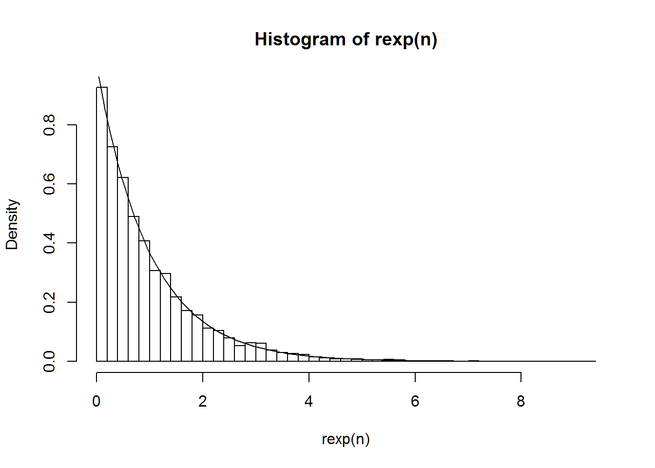
n = 1000
hist(rexp(n),breaks=35,freq=F)
curve(dexp,from=0,to=8,add=T) #add means add curve to previous plot.
#this is fun. Let's try it with fewer
n = 100
hist(rexp(n),breaks=35,freq=F)
curve(dexp,from=0,to=8,add=T) #add means add curve to previous plot.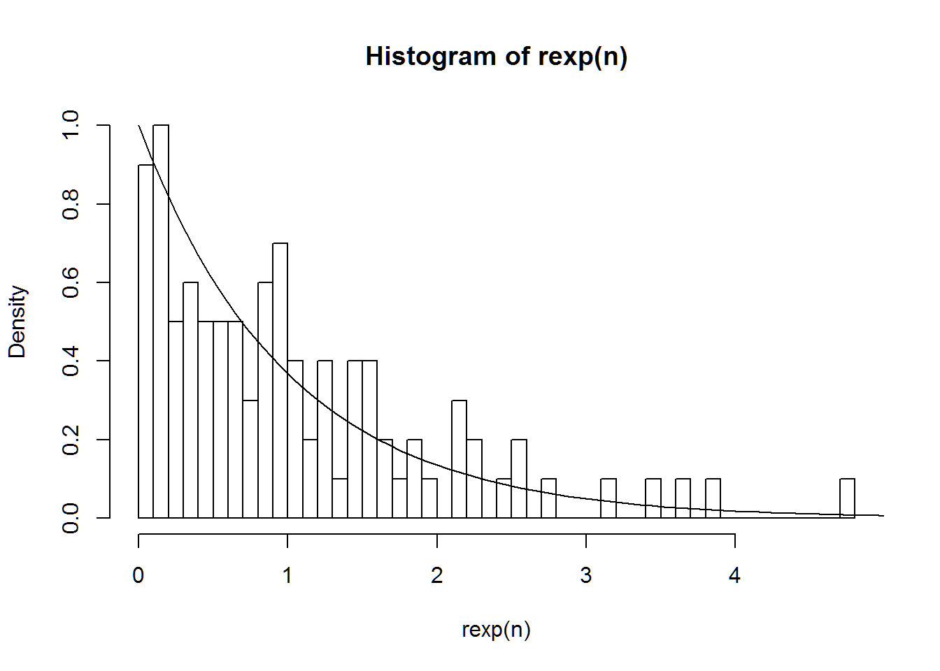
#this is fun. Let's try it with fewer
n = 10
hist(rexp(n),breaks=35,freq=F)
curve(dexp,from=0,to=8,add=T) #add means add curve to previous plot.
6 Frozen Yogurt
#a.  We have a few ways to do this
# all four give the same answer
1-pnorm(q=8.64,mean=8,sd=.5,lower.tail = TRUE)
## [1] 0.1002726pnorm(q=8.64,mean=8,sd=.5,lower.tail = FALSE)## [1] 0.1002726z = (8.64 - 8)/.5
# z is 1.28
1-pnorm(q=z)## [1] 0.1002726pnorm(q=z,lower.tail=FALSE)## [1] 0.1002726#b.
pnorm(q=z,lower.tail=FALSE)^3## [1] 0.0010081998 College Admissions
- Normal with μ = 500 and σ = 80.
- College A accepts all above 600.
- College B accepts the top 1%.
pnorm(600,500,80,lower.tail = FALSE)## [1] 0.1056498qnorm(.01,500,80,lower.tail=FALSE)## [1] 686.10789 Piston Rings
#a
# both give the same answer
qnorm(.8508,10,.03,lower.tail = FALSE)
## [1] 9.968804qnorm(1-.8508,10,.03,lower.tail = TRUE)## [1] 9.968804#b
pnorm(10.06,10,.03,lower.tail=TRUE)## [1] 0.977249911 QQ plots
See below for my comments on QQ plots
x= runif(50)
qqnorm(x)
qqline(x,col=2)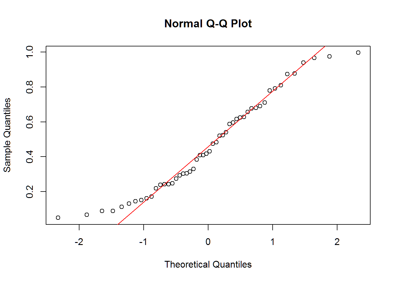
x= rgamma(50,1,1)
qqnorm(x)
qqline(x,col=2)
13ac Gamma Distribution (don’t do b)
In R the Gamma distribution matches the book with parameters shape = α = a and scale = β = s. Notice in R that the user can enter the rate or scale values and that the scale or β is $\frac{1}{rate}$.
## With a rate of 1 the scale is 1.
#a

# expected value is 1
curve(dgamma(x,shape=1,rate=1),from=0,to=7,ylab="Gamma PDFs")
# expected value is 2
curve(dgamma(x,shape=2,rate=1),from=0,to=7,add=T,col=2)
# expected value is 4
curve(dgamma(x,shape=4,rate=1),from=0,to=7,add=T,col=3)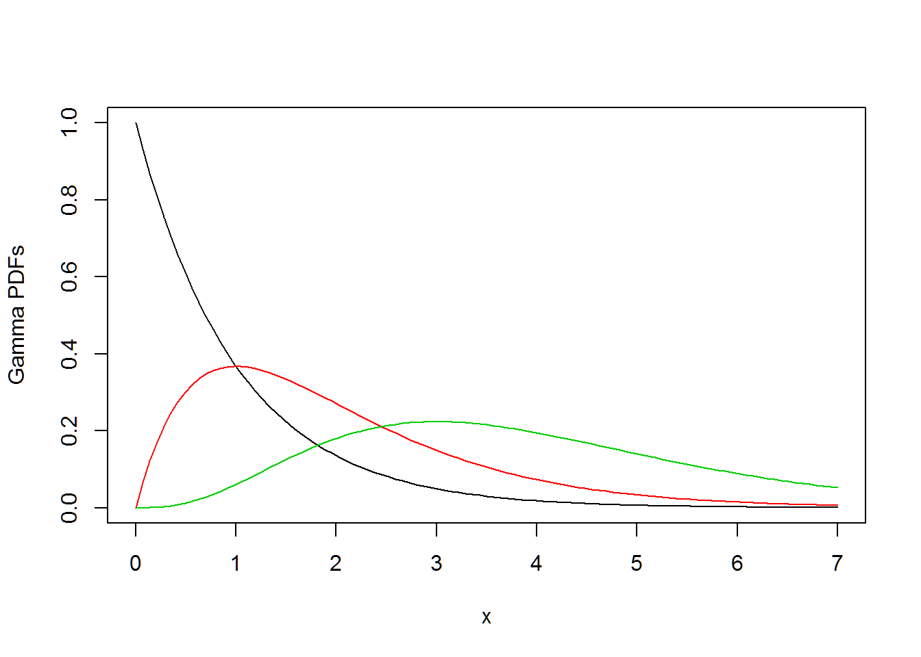
# we could work out the expectation through integration as well
integrate(function(x) x*dgamma(x,shape=4,rate=1),lower=0,upper=Inf)
## 4 with absolute error < 3.7e-06# expected value is 1
curve(pgamma(x,shape=1,rate=1),from=0,to=7,ylab="Gamma PDFs")
# expected value is 2
curve(pgamma(x,shape=2,rate=1),from=0,to=7,add=T,col=2)
# expected value is 4
curve(pgamma(x,shape=4,rate=1),from=0,to=7,add=T,col=3)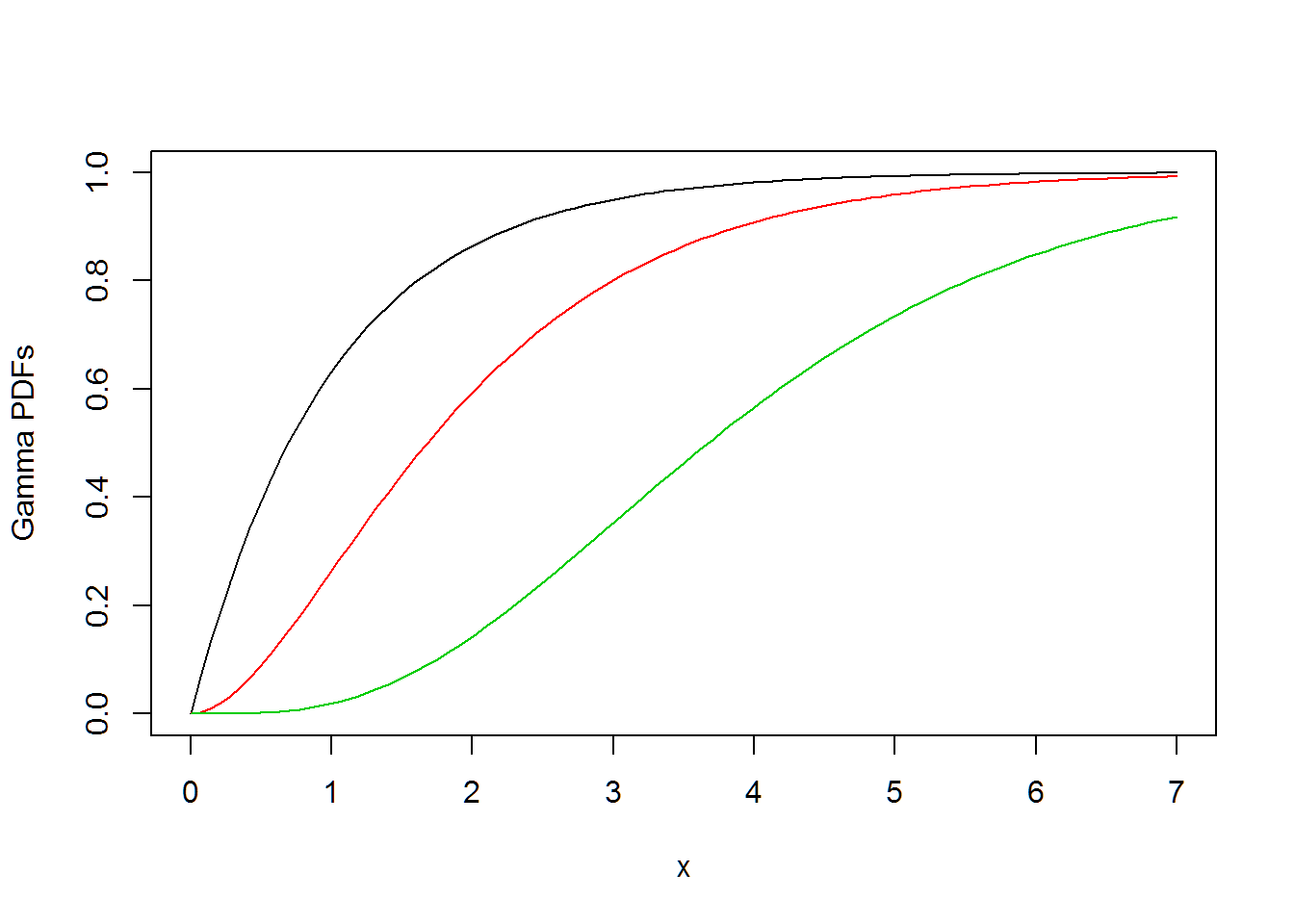
#c
qgamma(.95,shape=2,scale=1)
## [1] 4.743865qgamma(.95,shape=2,scale=2)## [1] 9.487729qgamma(.95,shape=3,scale=1)## [1] 6.295794qgamma(.95,shape=3,scale=2)## [1] 12.59159# These are the means for the two cases where the scale does not equal rate.
integrate(function(x) x*dgamma(x,shape=2,scale=2),lower=0,upper=Inf)## 4 with absolute error < 9.3e-05integrate(function(x) x*dgamma(x,shape=3,scale=2),lower=0,upper=Inf)## 6 with absolute error < 3.4e-05# the black vertical line is the mean. The read line is the 95th percentile.
curve(dgamma(x,shape=3,scale=2),from=0,to=18,ylab="Gamma PDFs")
abline(v=integrate(function(x) x*dgamma(x,shape=3,scale=2),lower=0,upper=Inf)$value)
abline(v=qgamma(.95,shape=3,scale=2),col=2)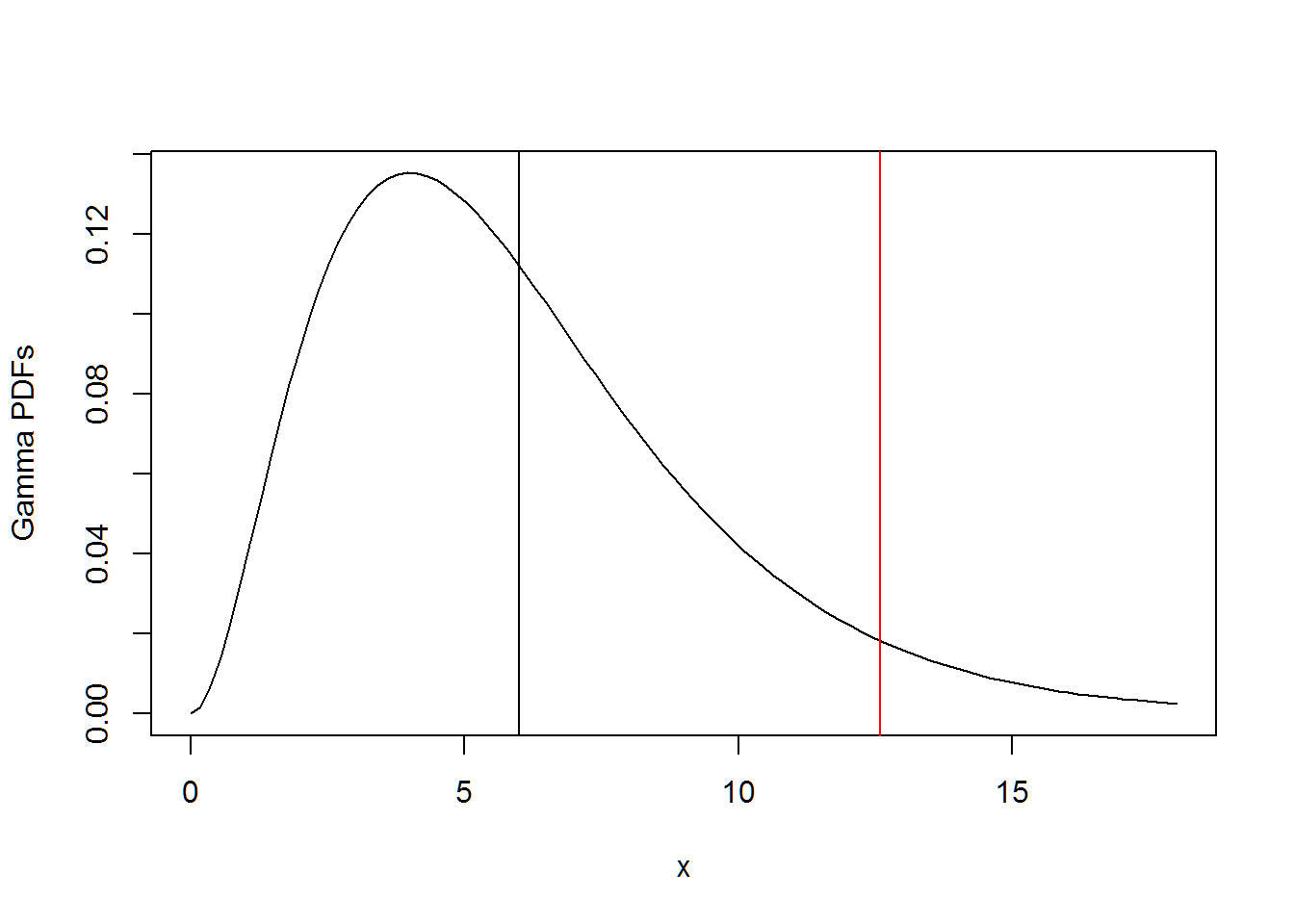
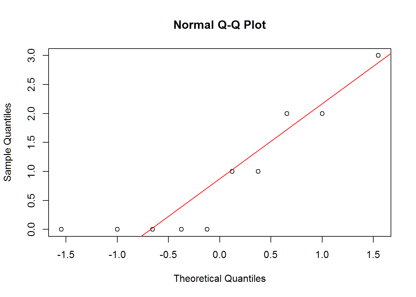
Notes on QQ plots
x= rgamma(10,1,1)
qqnorm(x)
qqline(x,col=2)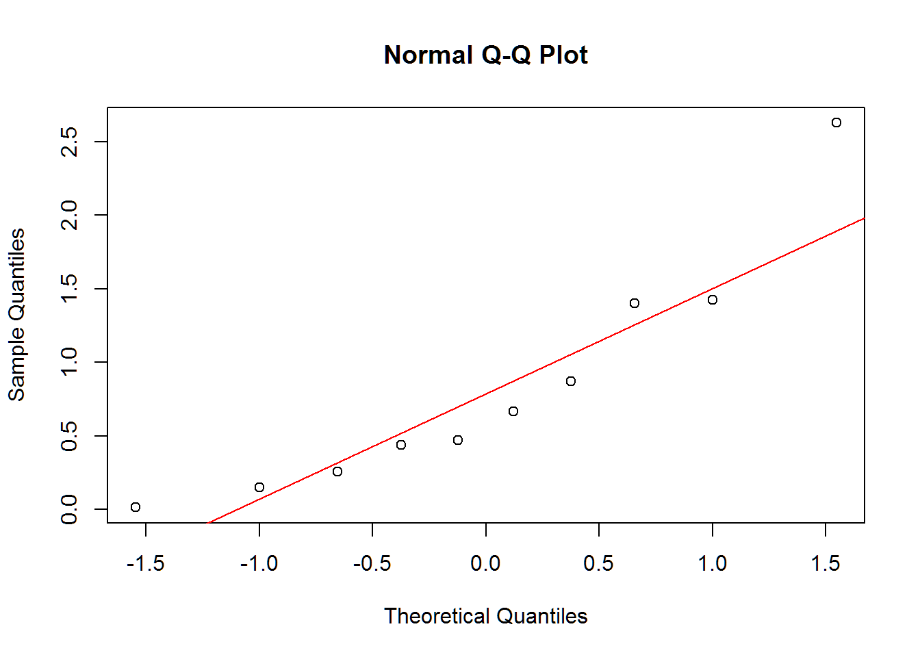
x= rnorm(10)
qqnorm(x)
qqline(x,col=2)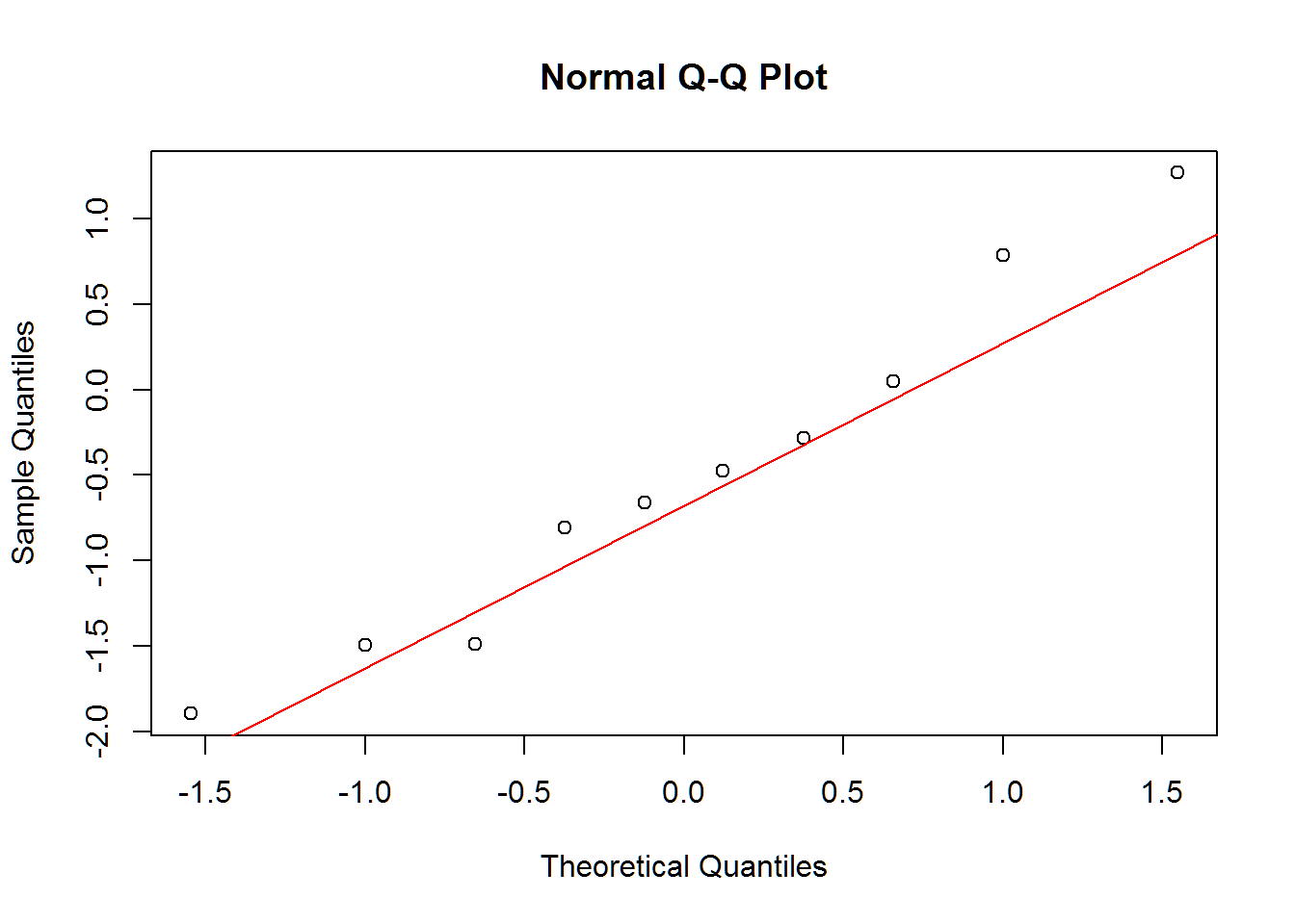
x= runif(10)
qqnorm(x)
qqline(x,col=2)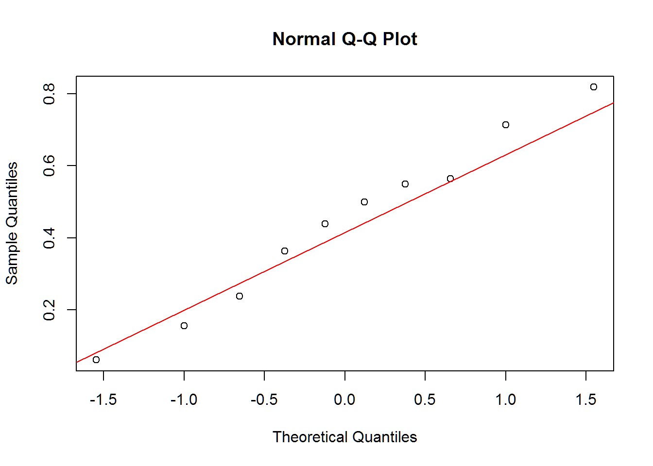
x= rpois(10,1)
qqnorm(x)
qqline(x,col=2)