ANOVA 10.2 and 10.3
The F-distribution
The following two plots match the plots shown in the Prezi class slides on ANOVA.
plot(seq(0,6,by=.1),df(seq(0,6,by=.1),4,12),type="l")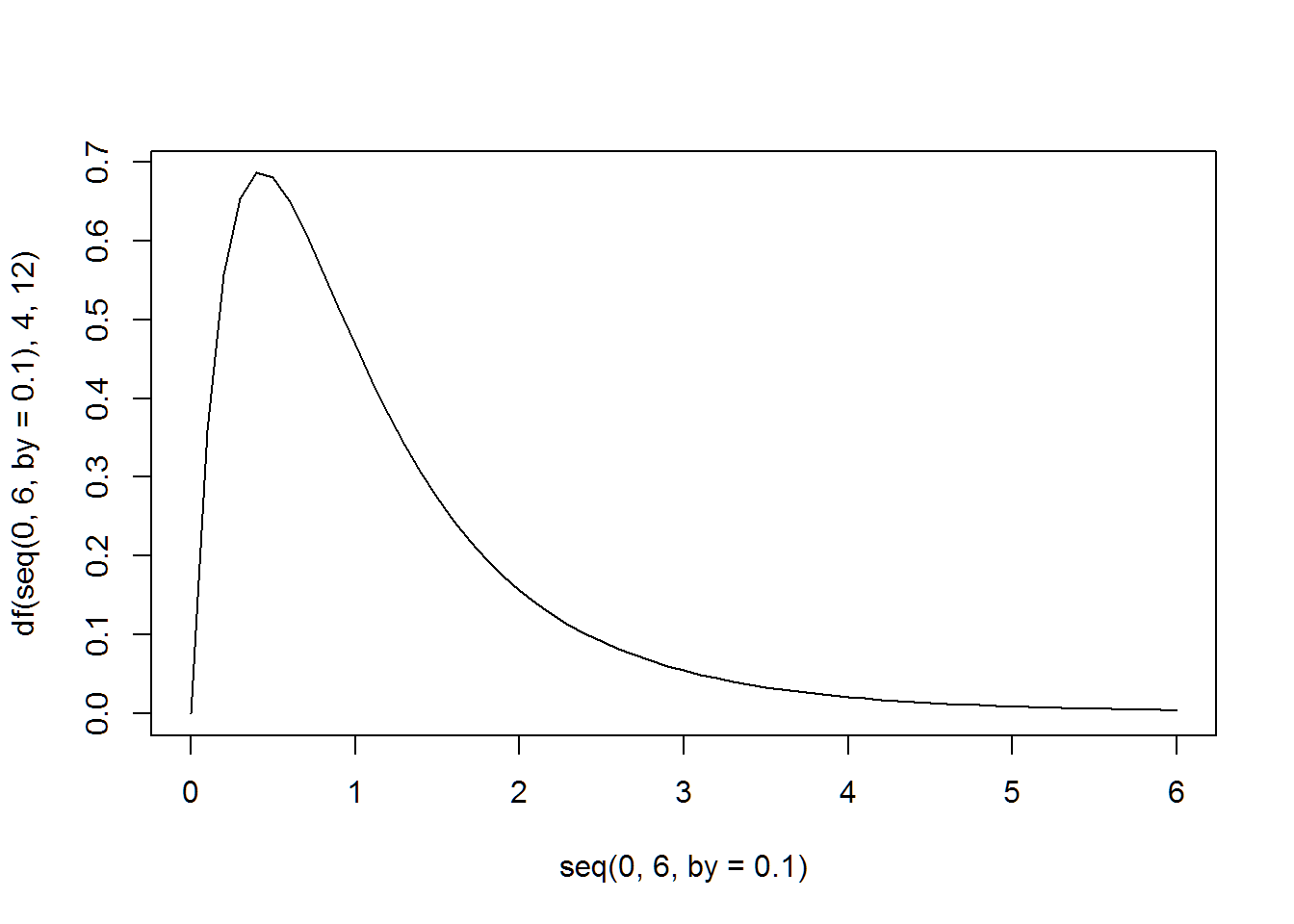
plot(seq(0,6,by=.1),df(seq(0,6,by=.1),10,100),type="l")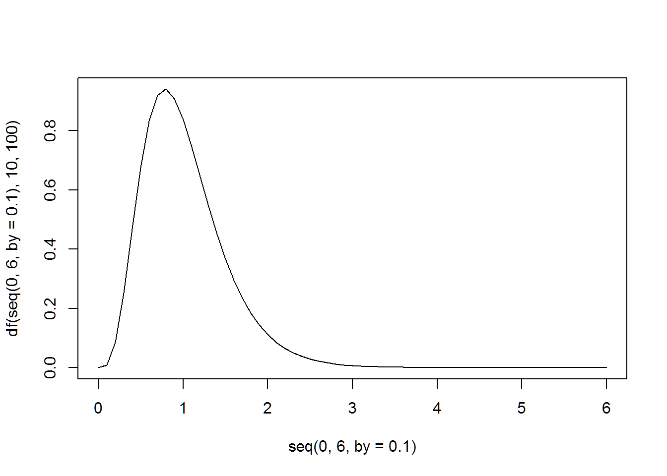
Your Job (Part 1)
- Use the code above (or below) and change the degrees of freedom to get a plot that looks like a normal distribution.
- After getting a plot that approximately normal follows a normal distribution, use the two degrees of freedom to describe how many groups and how many observations per group you would need in your experiment to result in this F-distribution that looks approximately normal.
- Now calculate the rejection rule for a three group experiment with 12 observations per group.
- In terms of an AOV test what would a large F-statistic from my study imply about my groups?
- Why does the F-distribution get less right skewed with more degrees of freedom?
# an example that doesn't have the right degrees of freedom
plot(seq(0,6,by=.1),df(seq(0,6,by=.1),5,65),type="l")
abline(v=qf(.95,5,65),col="red")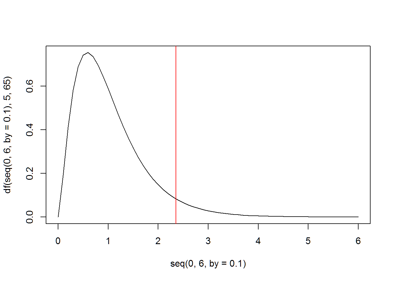
Analysis of Variance Example
We are going to use the leveneTest in the car library. Use install.pacakges("car") to get this package. This function will replace the code shown in Akritas on pg 352 for testing homogeneity of variance. The code below will show the book example the the method using leveneTest.
I can’t quite get the book to match the leveneTest function, but I would trust the leveneTest function over the books notation. If would like to see the details read here or here. Here are a few R examples on the different tests for homogeneity of variance.
#install.packages("car")
library(car)
library(DT)
library(ggplot2)
library(plyr)
# example starts on pg 350 in Akritas
data.dir = "http://media.pearsoncmg.com/cmg/pmmg_mml_shared/mathstatsresources/Akritas"
wq = read.table(file.path(data.dir,"WaterQualityIndex.txt"),header=T)
wq$Beach = as.factor(wq$Beach)

wq.aov = aov(Index~Beach,data=wq)
wq.anova = anova(wq.aov)

# The books method for testing equality of variance based on the mean.
anova(aov(resid(aov(Index~Beach,data=wq))**2~wq$Beach))
## Analysis of Variance Table
##
## Response: resid(aov(Index ~ Beach, data = wq))^2
## Df Sum Sq Mean Sq F value Pr(>F)
## wq$Beach 4 1.2232 0.30579 1.6854 0.1665
## Residuals 55 9.9789 0.18144# These are what we will use. This levene test is based on the median wich is more robust to departures from normality.
bartlett.test(Index~Beach,data=wq)##
## Bartlett test of homogeneity of variances
##
## data: Index by Beach
## Bartlett's K-squared = 4.3538, df = 4, p-value = 0.3602leveneTest(Index~Beach,data=wq,center="mean")## Levene's Test for Homogeneity of Variance (center = "mean")
## Df F value Pr(>F)
## group 4 1.8067 0.1407
## 55leveneTest(Index~Beach,data=wq,center="median")## Levene's Test for Homogeneity of Variance (center = "median")
## Df F value Pr(>F)
## group 4 1.2756 0.2907
## 55leveneTest(wq.aov)## Levene's Test for Homogeneity of Variance (center = median)
## Df F value Pr(>F)
## group 4 1.2756 0.2907
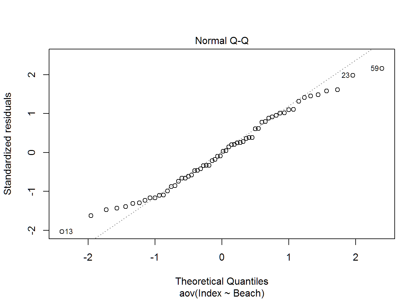
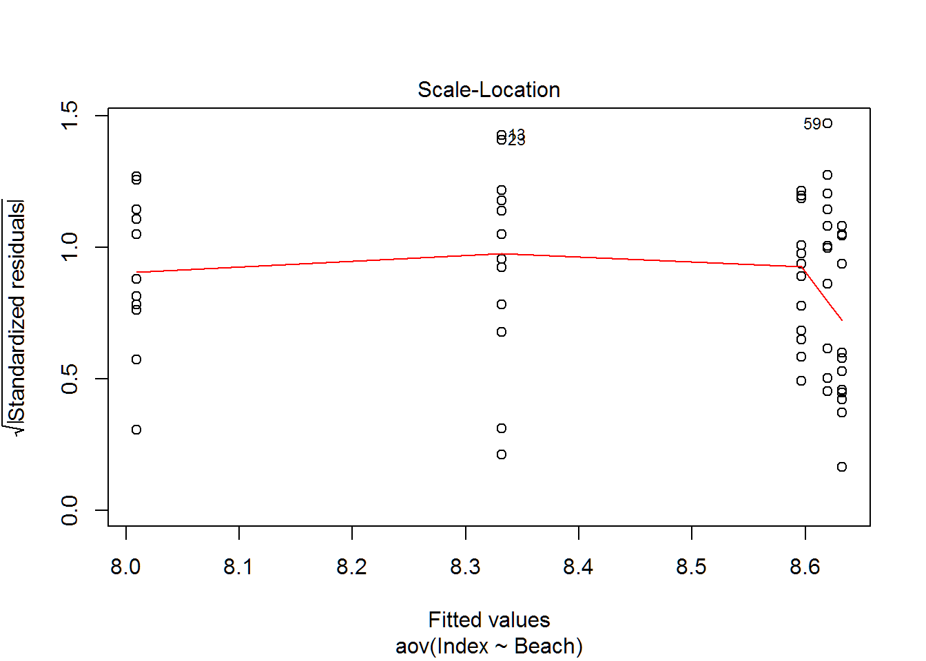
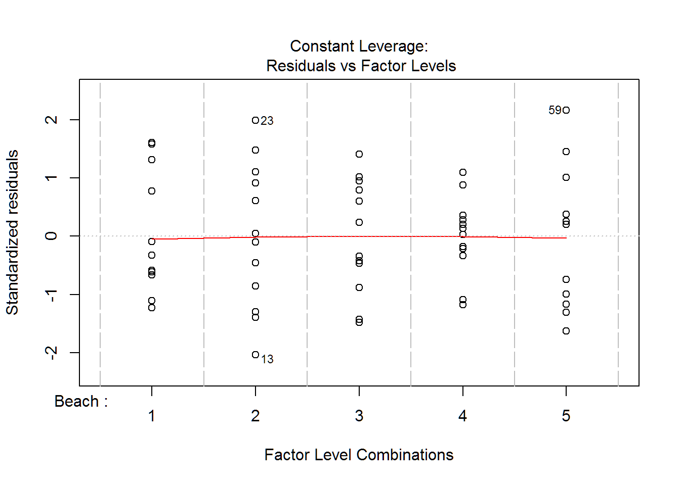
## 55shapiro.test(resid(wq.aov))##
## Shapiro-Wilk normality test
##
## data: resid(wq.aov)
## W = 0.97996, p-value = 0.427#shapiro.test(wq.aov$residuals)
plot(wq.aov)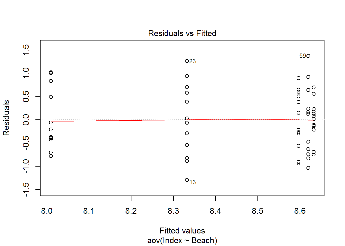
Multiple Comparisons
TukeyHSD(wq.aov)## Tukey multiple comparisons of means
## 95% family-wise confidence level
##
## Fit: aov(formula = Index ~ Beach, data = wq)
##
## $Beach
## diff lwr upr p adj
## 2-1 0.32250000 -0.4401421 1.0851421 0.7555222
## 3-1 0.58750000 -0.1751421 1.3501421 0.2054300
## 4-1 0.62333333 -0.1393088 1.3859755 0.1587930
## 5-1 0.61083333 -0.1518088 1.3734755 0.1740616
## 3-2 0.26500000 -0.4976421 1.0276421 0.8631067
## 4-2 0.30083333 -0.4618088 1.0634755 0.7992641
## 5-2 0.28833333 -0.4743088 1.0509755 0.8228381
## 4-3 0.03583333 -0.7268088 0.7984755 0.9999282
## 5-3 0.02333333 -0.7393088 0.7859755 0.9999870
## 5-4 -0.01250000 -0.7751421 0.7501421 0.9999989plot(TukeyHSD(wq.aov))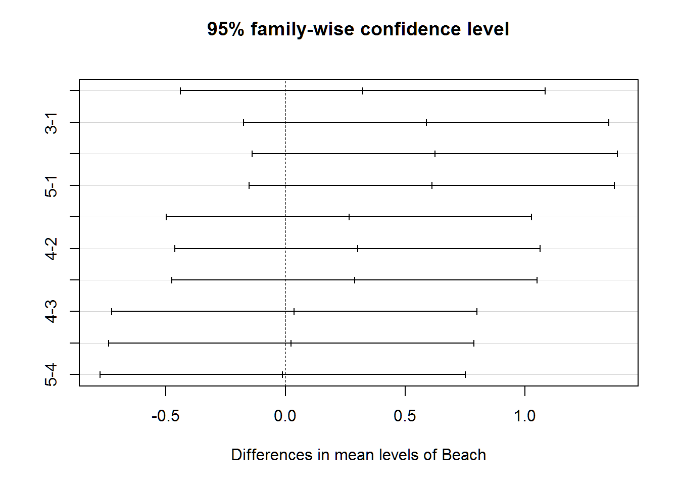
Your Job (Part 2)
Use this hot dog data to decide which type of hot dog is the healthiest.
- Make sure you check your assumptions. Show the plots and test results.
- You are going to use
shapiro.test(resid(wq.aov))for normality andleveneTest(Index~Beach,data=wq,center="median")for equal variance. - Remember to read the Prezi for Unit 10 on Robustness.
- You are going to use
- Perform the ANOVA test.
- Do the multiple comparison to decide which type is the healthiest.
- Provide an informative plot of the groups that shows your results.
- Write a one paragraph conclusion from your study that could be used on a newspaper article (meaning that normal people would read and understand).
Your Job (Part 3)
It turns out that people actually do studies on efficacy of antiperspirants. The journal of Cosmetological Chemistry published and article on The Evaluation of Antiperspirant Efficacy–Influence of Certain Variables which documents the data that we will used below. This data and many other data sets can be found here. The code chunk below will read the data into R. Four different brands of deodorant were examined for their efficacy in reduction of perspiration. They have asked you to perform that statistical analysis.
- Make sure you check your assumptions (use the Prezi text). Show the plots and test results. * You are going to use
shapiro.test(resid(sweat.aov))for normality andleveneTest(SR~Brand,data=sweat,center="median")for equal variance. - Perform the ANOVA test.
- Do the multiple comparison to decide which type is the healthiest.
- Provide an informative plot of the groups that shows your results.
- Write a one paragraph conclusion from your study that could be used on their article (meaning that normal people would read and understand).
sweat = read.table(file="http://www.stat.ufl.edu/~winner/data/sweat_reduction.dat",col.names = c("Subject","Brand","SR"))
sweat$Subject = as.factor(sweat$Subject)
sweat$Brand = as.factor(sweat$Brand)
sweat.aov= aov(SR~Brand+Subject,data=sweat)
anova(sweat.aov)

ggplot(data=sweat,aes(x=Brand,y=SR))+
  geom_boxplot()+
  geom_jitter(height=0)

ggplot(data=sweat,aes(x=Brand,y=SR))+
  geom_boxplot()+
  geom_jitter(aes(color=Subject),height=0)

ggplot(data=sweat,aes(x=Subject,y=SR))+
  geom_jitter(aes(color=Brand),height=0)

smean = ddply(.data=sweat,.variables=.(Subject),.fun=function(x){
      data.frame(Subject_mean = mean(x$SR))
      })
bmean = ddply(.data=sweat,.variables=.(Brand),.fun=function(x){
      data.frame(Brand_mean = mean(x$SR))
      })
omean = mean(sweat$SR)

smean$Subject = as.numeric(as.character(smean$Subject))
sweat$Subject_Num = as.numeric(as.character(sweat$Subject))

no_block_plot = ggplot(data=sweat)+
  geom_hline(yintercept=omean,size=1.4)+
  geom_hline(data=bmean,aes(yintercept=Brand_mean,colour=Brand,lty=Brand),size=1.4)+
  scale_x_continuous(breaks=1:24)+
  theme_bw()+labs(x="Subject",y="Sweat Reduction")

no_block_plot +  facet_wrap(~Brand) +   geom_point(aes(x=Subject_Num,y=SR,colour=Brand,shape=Brand),size=1.5)


no_block_plot + geom_segment(data=smean,size=1.4,colour="orange",
               aes(x=Subject-.5,xend=Subject+.5,y=Subject_mean,yend=Subject_mean))+
   geom_jitter(aes(x=Subject_Num,y=SR,colour=Brand,shape=Brand),width=.35,height=0,size=1.5)

no_block_plot + geom_segment(data=smean,size=1.4,colour="orange",
               aes(x=Subject-.5,xend=Subject+.5,y=Subject_mean,yend=Subject_mean))+
   geom_jitter(aes(x=Subject_Num,y=SR,colour=Brand,shape=Brand),width=.35,height=0,size=1.5)+  facet_wrap(~Brand)


plot(TukeyHSD(sweat.aov,"Brand"))