Example 1.8-4

data.dir = "http://media.pearsoncmg.com/cmg/pmmg_mml_shared/mathstatsresources/Akritas"
fe = read.table(file.path(data.dir,"FeData.txt"),header=T)

# Akritas Code
# don't use this
#w = stack(fe)
boxplot(fe$conc~fe$ind)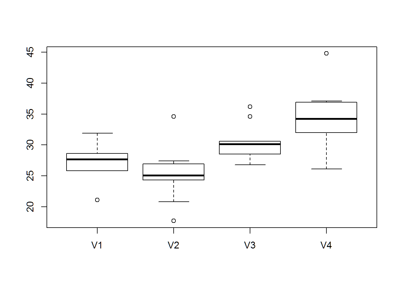

# Hathaway ggplot2 Example
library(ggplot2)
ggplot(data=fe,aes(x=ind,y=conc))+geom_boxplot()+theme_bw()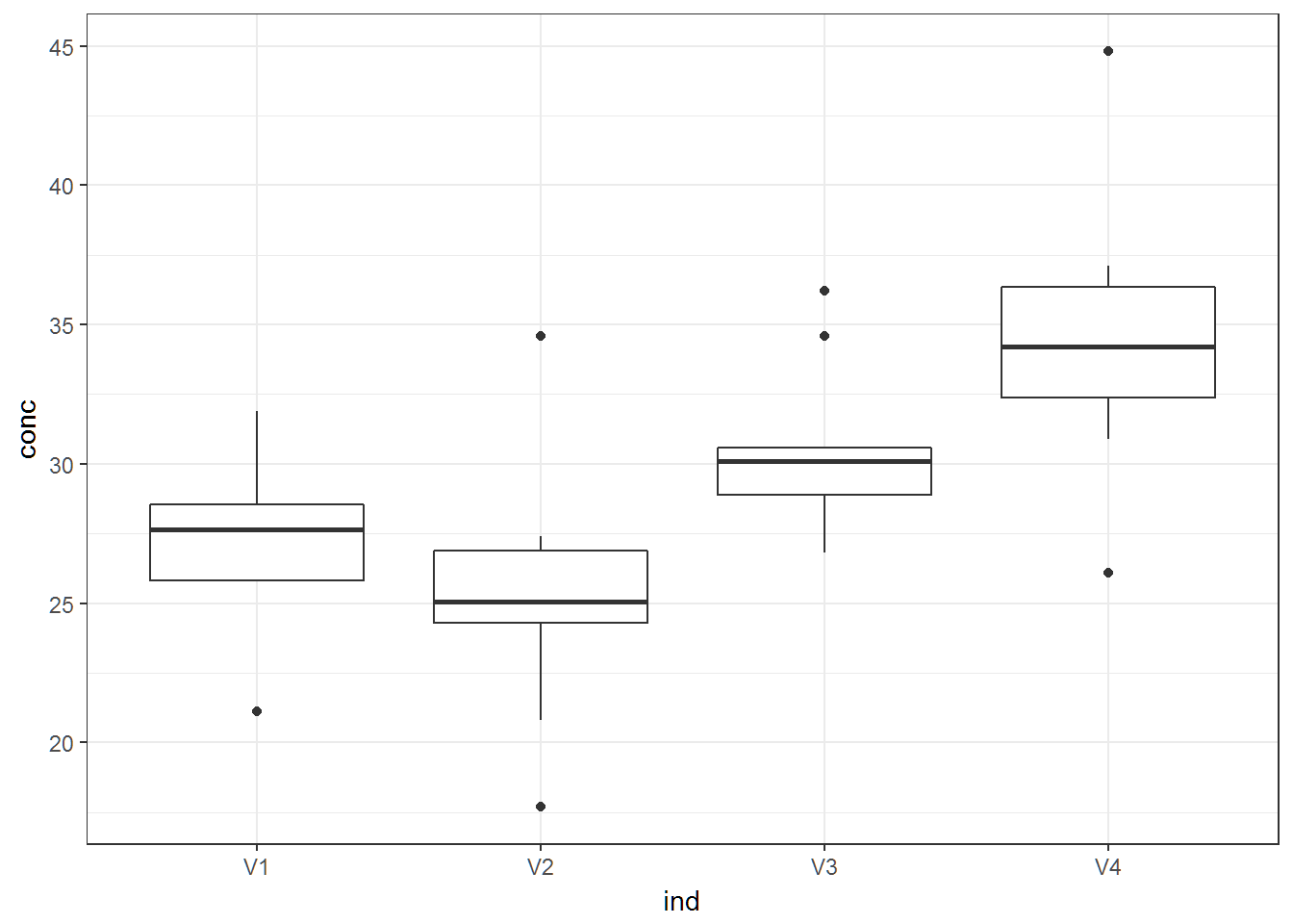

Example 1.8.5

lv2 = read.table(file.path(data.dir,"MarketShareLightVehComp.txt"),header=T)
# Akritas Code
m=rbind(lv2$Percent_2010,lv2$Percent_2011)
barplot(m,names.arg=lv2$Company,beside=T,las=2)

# Hathaway code
library(reshape)

## Warning: package 'reshape' was built under R version 3.3.1

# Create long format data
lv2_melt = melt(lv2,id.vars = "Company")
ggplot(data=lv2_melt,aes(x=Company,y=value,fill=variable))+
  geom_bar(position="dodge",stat="identity")+
  coord_flip()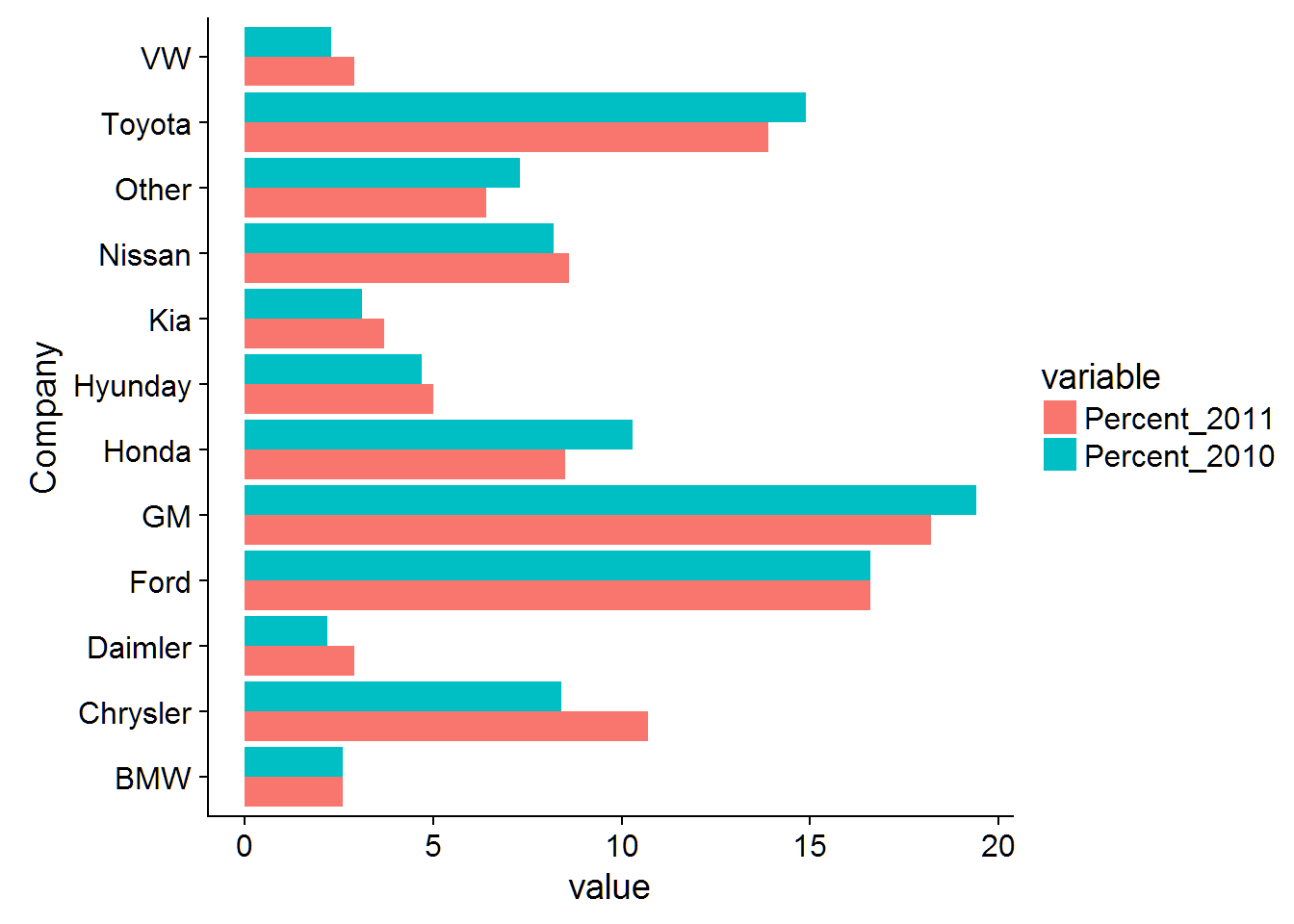

Example 1.8-6

Note that the file is named wrong in the book. The book says QsalesSphone.txt and even the hyperlink on the data page says the same. However, the actual name is QsalesIphone.txt

qs = read.table(file.path(data.dir,"QsalesIphone.txt"),header=T)
# akritas code
m = rbind(qs$Q1,qs$Q2,qs$Q3,qs$Q4)
barplot(m, names.arg=qs$Year, ylim=c(0,40000),col=c("green","blue","yellow","red"))
legend("topleft",pch=rep(22,4),pt.bg=c("green","blue","yellow","red"),legend = paste("Quarter",1:4))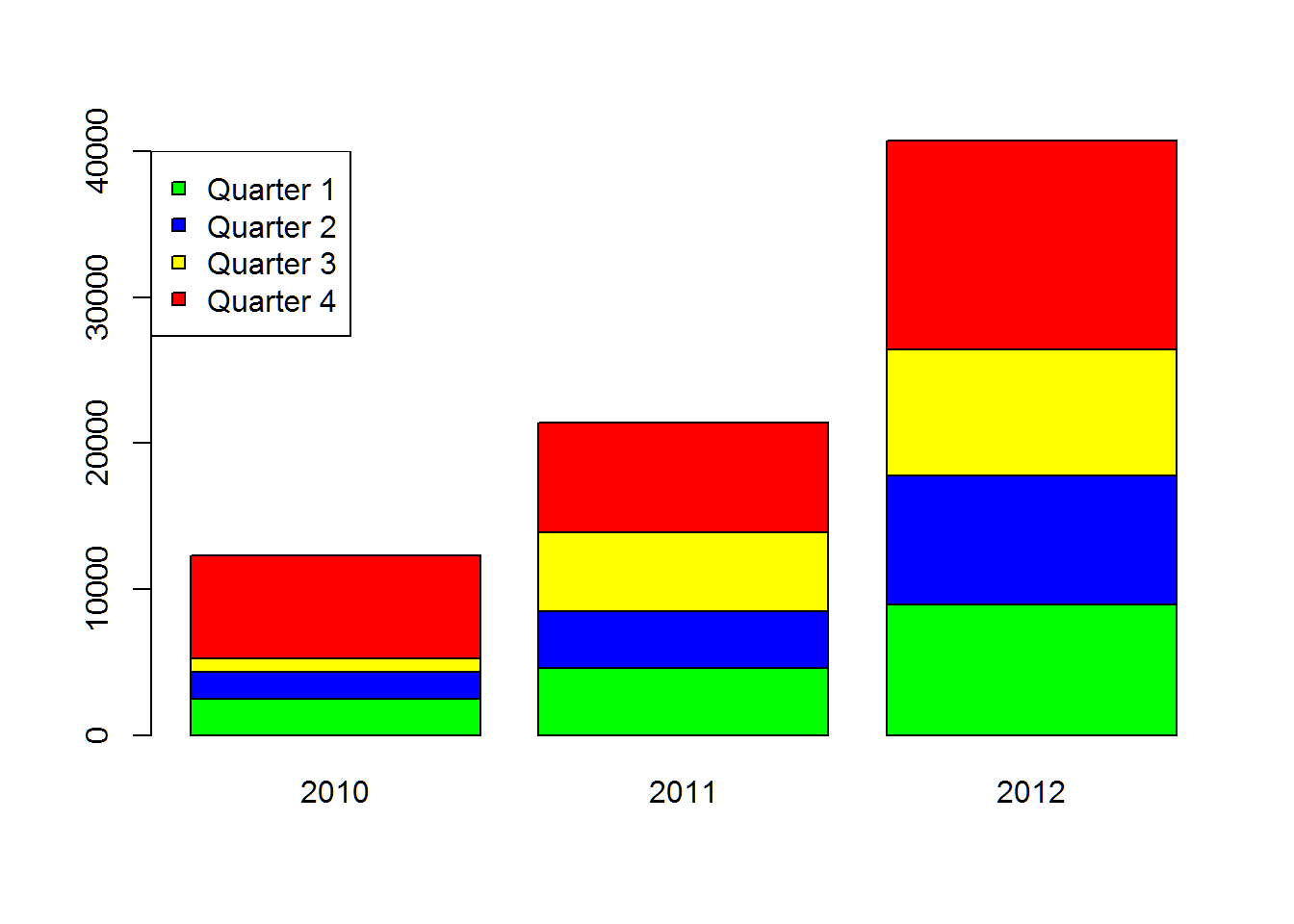

# Hathaway code
# I try to avoid stacked bar charts.  This one isn't too bad.
library(ggplot2)
library(reshape)
ggplot(data=melt(qs,id.vars="Year"))+
  geom_bar(aes(x=Year,y=value,fill=variable),stat="identity",colour="black")+
  theme_bw()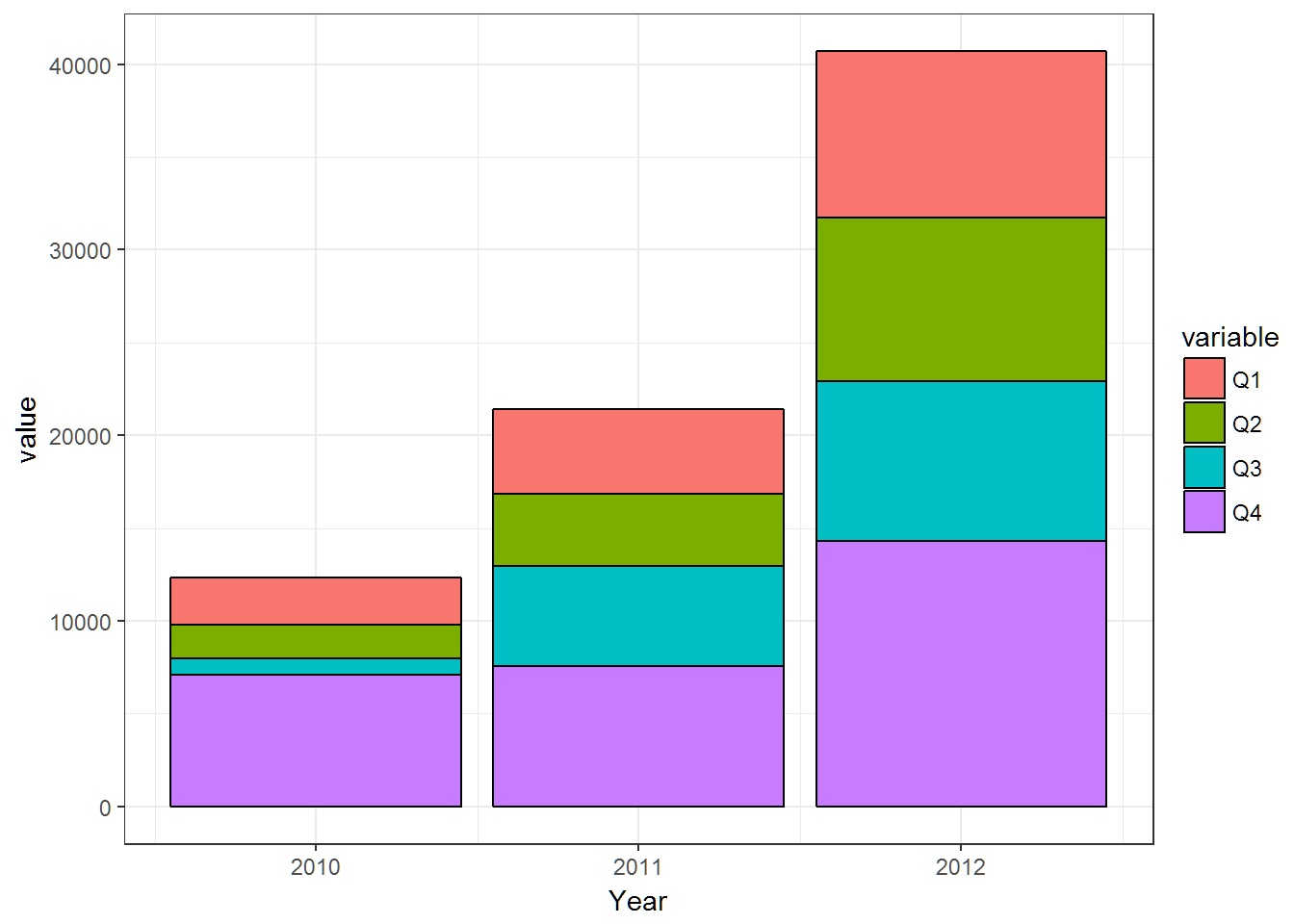

Example 1.8-12

cs = read.table(file.path(data.dir,"CloudSeed2w.txt"),header=T)
# akritas code
interaction.plot(cs$season,cs$seeded,cs$rain,col=c(2,3),lty=1,xlab="Season",ylab="Cell Means of Rainfall",trace.label = "Seeding")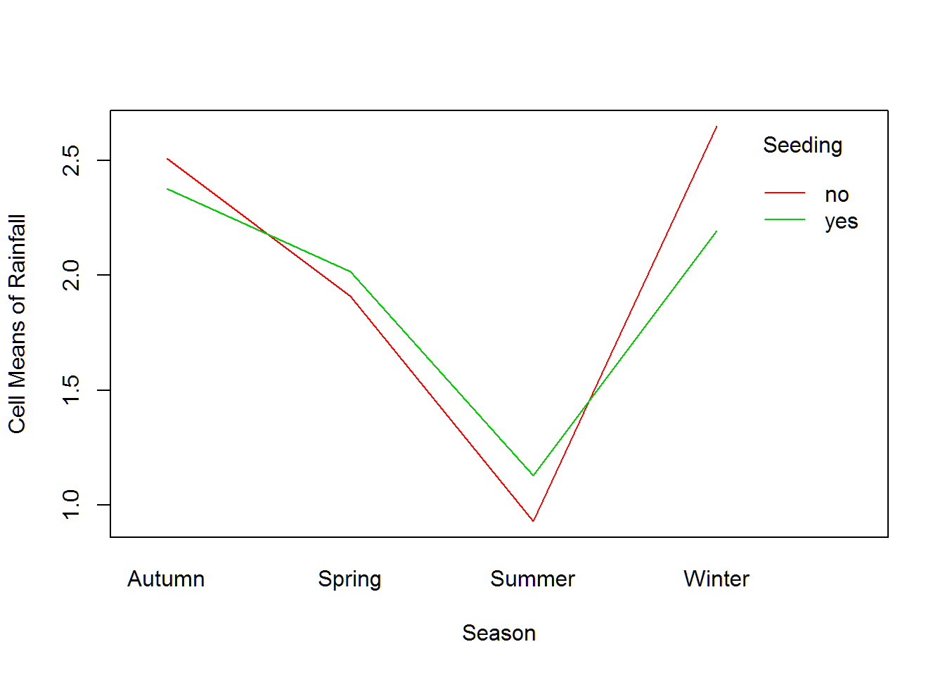

# Hathaway code
ggplot(data=cs,aes(x=season,y=rain,fill=seeded))+
  geom_boxplot()+
  stat_summary(fun.y="mean",geom="point",shape=21,size=5)+theme_bw()

# Not sure we should be declaring interactions with the heavy overlap 
# and only 16 observations between groups, but there may be some interaction effect with seeding and winter...
table(cs$season)

## 
## Autumn Spring Summer Winter 
##     16     16     16     16