1.6-1.7 Homework

9 Dice

Here is how I would program the solution to this answer. This video shows the variance calcluation for a discrete probability distribution.

dice_sides = 1:6
prob_side = rep(1/6,6)
dice_mean = sum(dice_sides*prob_side)
# could use this as well
#dice_mean = mean(dice_sides)

# Here is the population variance for discrete probabilities which is a variation of equation 1.6.9
sum(dice_sides^2*prob_side)-dice_mean^2

## [1] 2.916667

# or using Equation 1.6.8
sum((dice_sides-dice_mean)^2)/length(dice_sides)

## [1] 2.916667

# Why does using the var command not give the same answer
var(dice_sides)

## [1] 3.5

# because var is doing the calculation for a sample not a population
sum((dice_sides-dice_mean)^2)/(length(dice_sides)-1)

## [1] 3.5

x = sample(1:6,100,replace=T)
mean(x)

## [1] 3.79

var(x)

## [1] 2.874646

# why are the mean and variance so much closer to the truth than the proportion estimates?
table(x)/100

## x
##    1    2    3    4    5    6 
## 0.14 0.12 0.15 0.19 0.20 0.20

# What is the difference between the line below and the question in number 9?
table(sample(1:6,600,replace=T))/600

## 
##         1         2         3         4         5         6 
## 0.1500000 0.1583333 0.1600000 0.1833333 0.1883333 0.1600000

11 Gas Mileage

acars = c(29.1,29.6,30,30.5,30.8)
bcars = c(21,26,30,35,38)

#a 
mean(acars)

## [1] 30

mean(bcars)

## [1] 30

#b
var(acars)

## [1] 0.465

var(bcars)

## [1] 46.5

13

This is a paper and pencil problem see

14

This is a paper and pencil problem and depends on the work in problem 13

16 Salaries

sal = c(152,169,178,179,185,188,195,196,198,203,204,209,210,212,214)
# a
mean(sal)

## [1] 192.8

var(sal)

## [1] 312.3143

# and sd
sd(sal)

## [1] 17.67242

# b 
# We could use results from problem 13 or just change the sal data and calculate mean and var again
sal2 = sal+5
mean(sal2)

## [1] 197.8

var(sal2)

## [1] 312.3143

sal3 = sal*1.05
mean(sal3)

## [1] 202.44

var(sal3)

## [1] 344.3265

2 Robot

data.dir = "http://media.pearsoncmg.com/cmg/pmmg_mml_shared/mathstatsresources/Akritas"
t = read.table(file.path(data.dir,"RobotReactTime.txt"),header=T)
t1 = t$Time[t$Robot==1]

sort(t1)

##  [1] 28.35 28.98 29.06 29.25 29.32 29.59 29.76 29.84 30.03 30.28 30.34
## [12] 30.76 30.84 31.01 31.19 31.27 31.41 31.55 31.60 31.90 32.42 32.74

3 Robot

t2 = t$Time[t$Robot==2]

sort(t2)

##  [1] 28.97 28.98 29.07 29.15 29.18 29.28 29.34 29.36 29.54 29.80 29.90
## [12] 29.98 30.54 30.66 30.78 30.80 30.83 30.86 30.87 31.09 31.18 32.23

summary(t2)

##    Min. 1st Qu.  Median    Mean 3rd Qu.    Max. 
##   28.97   29.30   29.94   30.11   30.82   32.23

quantile(t2,.9)

##    90% 
## 31.068

boxplot(t2)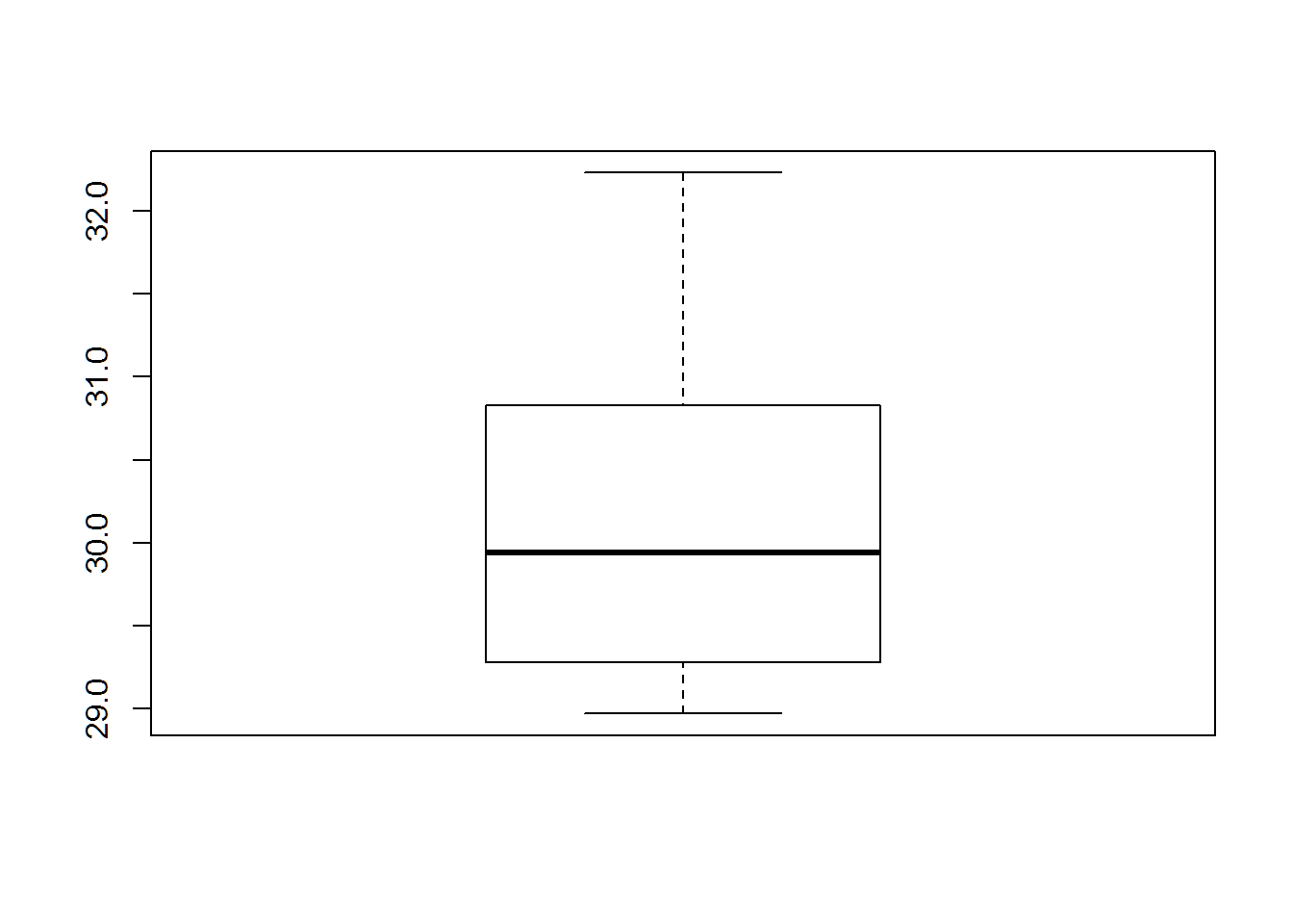

library(ggplot2)
ggplot(data=t,aes(x=as.factor(Robot),y=Time))+geom_boxplot()+theme_bw()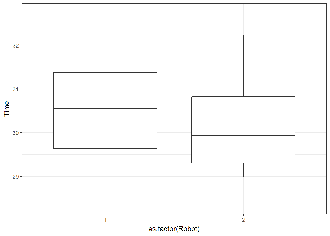

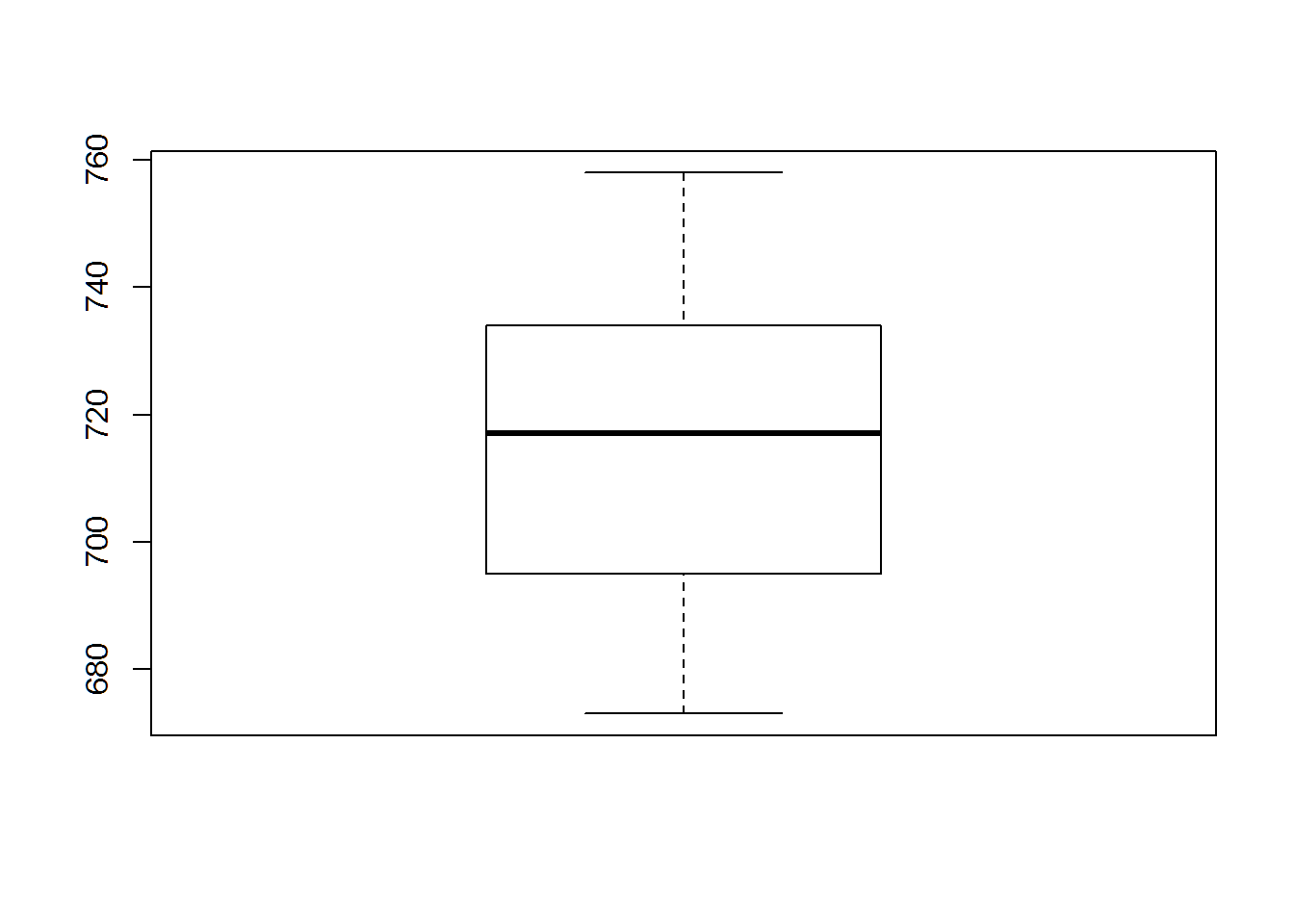
4 Solar

si = read.table(file.path(data.dir,"SolarIntensAuData.txt"),header=T)


quantile(si$SI,c(.3,.6,.9))

##   30%   60%   90% 
## 700.7 720.8 746.0

boxplot(si$SI)