1.5 Graphs for Understanding
- 1.5: 8-10,12-13 will be done in class (not due)
- 1.5: 1-4,6:7,11,16,17 (these are the ones you grade)
Class Problems
Please note that we are being a little loose with axis labels. As we are just learning R code lets not worry about it right now. However, labelling is vital for your tests and projects.
8 Age of Trees
data.dir = "http://media.pearsoncmg.com/cmg/pmmg_mml_shared/mathstatsresources/Akritas"
#8 Age of Trees
ad = read.table(file.path(data.dir,"TreeDiamAAge3Stk.txt"),header=T)
# code from Akritas
# notice that his example on pg 17 uses col in the legend.  He should be using pt.bg
with(ad,{
  plot(diam,age,pch=21,bg=c("red","green","blue")[unclass(tree)])
  legend(x=35,y=250,pch=c(21,21,21), pt.bg=c("red","green","blue"),legend=c("SMaple","ShHickory","WOak"))
})
# hathaway code with ggplot2
#install.packages("ggplot2")
library(ggplot2)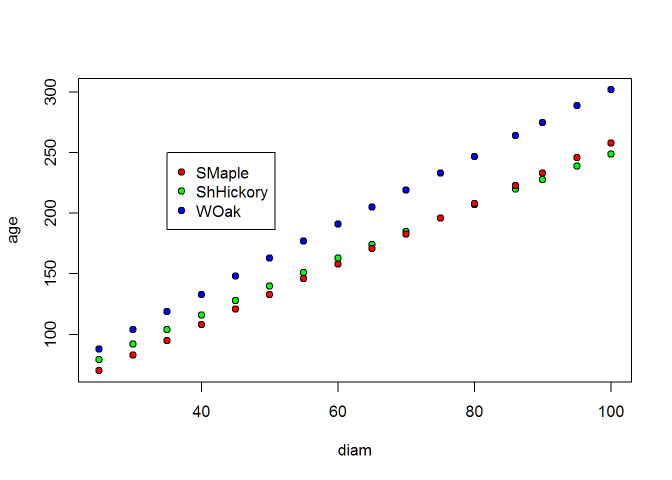
qplot(data=ad,x=diam,y=age,colour=tree,size=I(2.5))+theme_bw()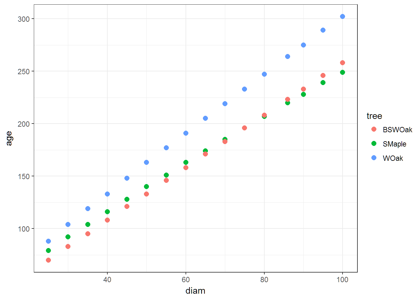
9 Robots
t = read.table(file.path(data.dir,"RobotReactTime.txt"),header=T)
t1 = t$Time[t$Robot==1]
# Akritas code
hist(t1,freq=FALSE,breaks=8)
lines(density(t1),col="red")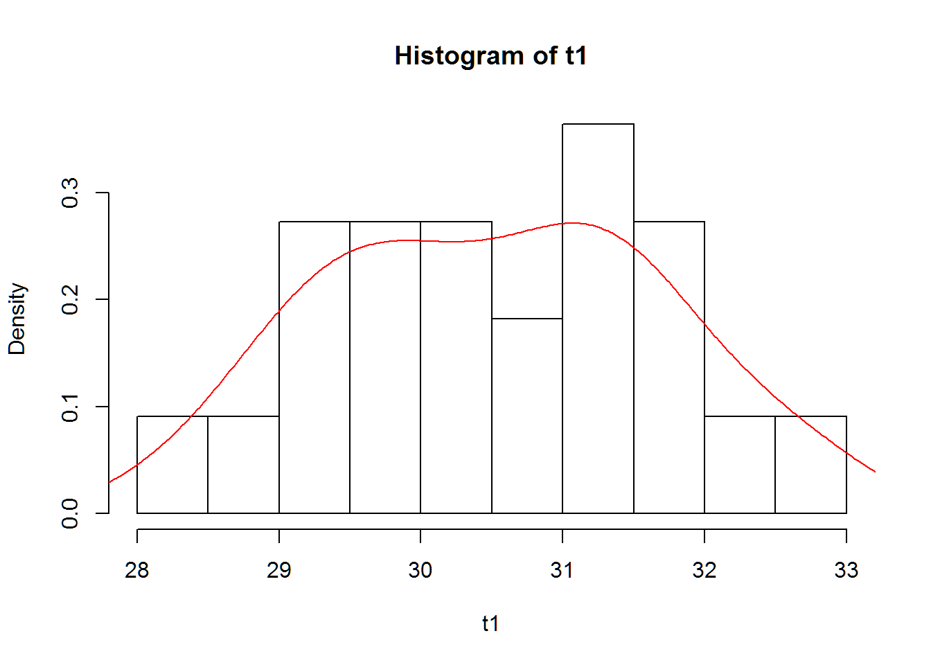
stem(t1)##
## The decimal point is at the |
##
## 28 | 4
## 29 | 0133688
## 30 | 03388
## 31 | 0234669
## 32 | 47# Hathaway code
qplot(x=t1,colour=I("white"),bins=8)+theme_bw()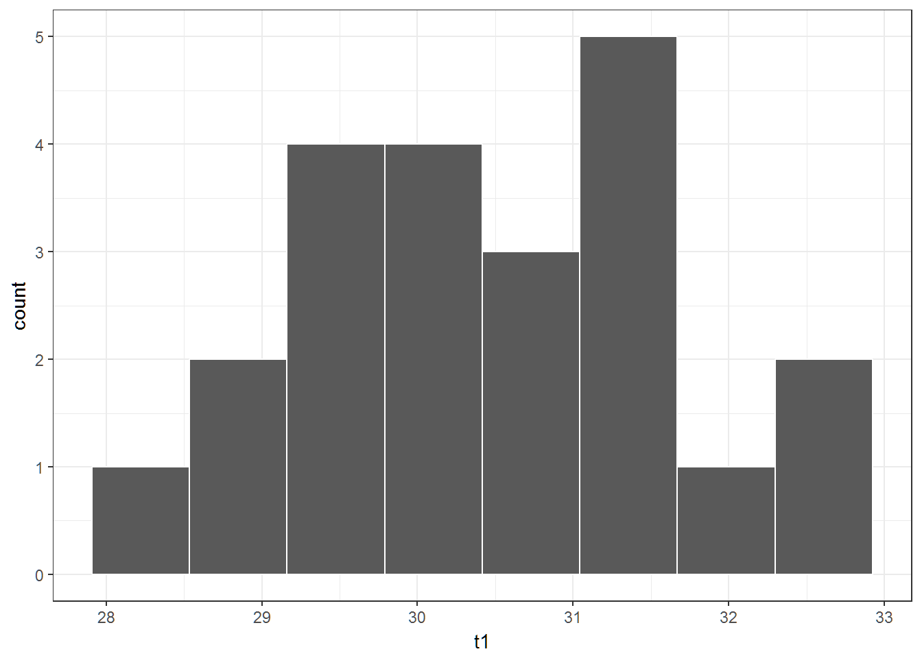
qplot(x=t1,colour=I("black"),geom="density")+theme_bw()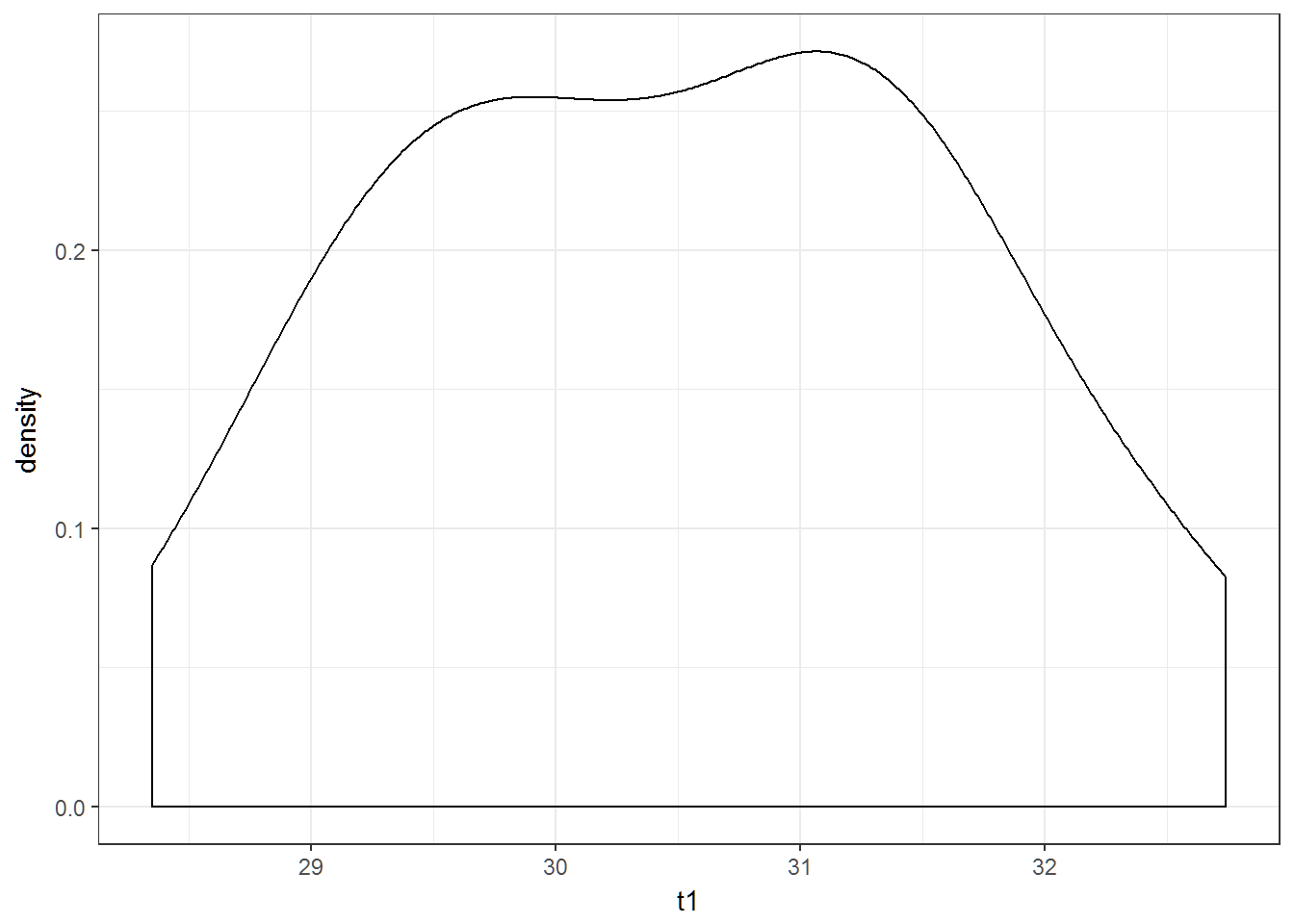
# Generally I would plot the density line or the histogram.  Not both.
ggplot(subset(t,Robot==1), aes(x=Time)) +
    geom_histogram(aes(y=..density..),bins=8, colour="black")+
    geom_density(adjust=1,colour="red",size=1.5)+theme_bw()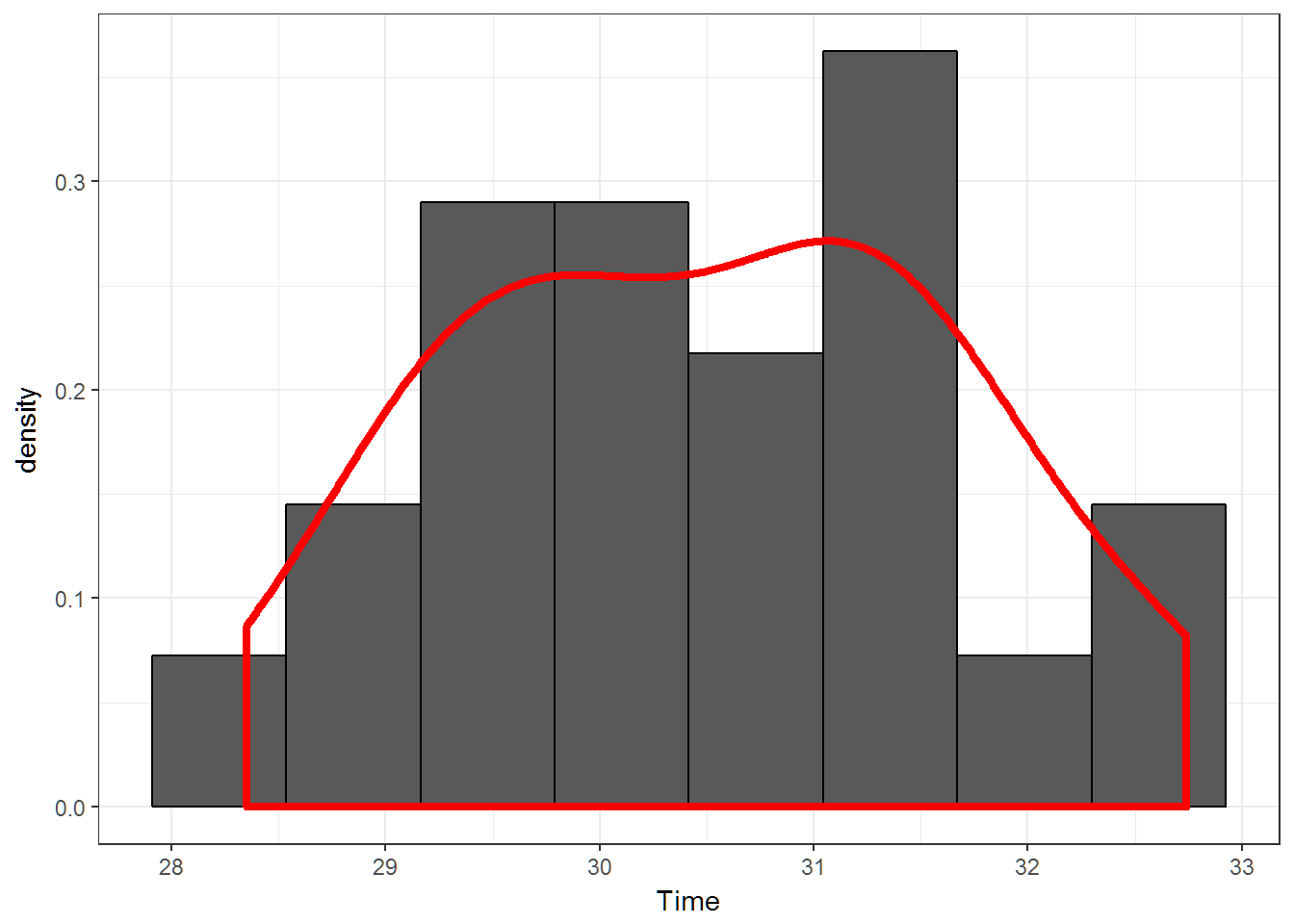
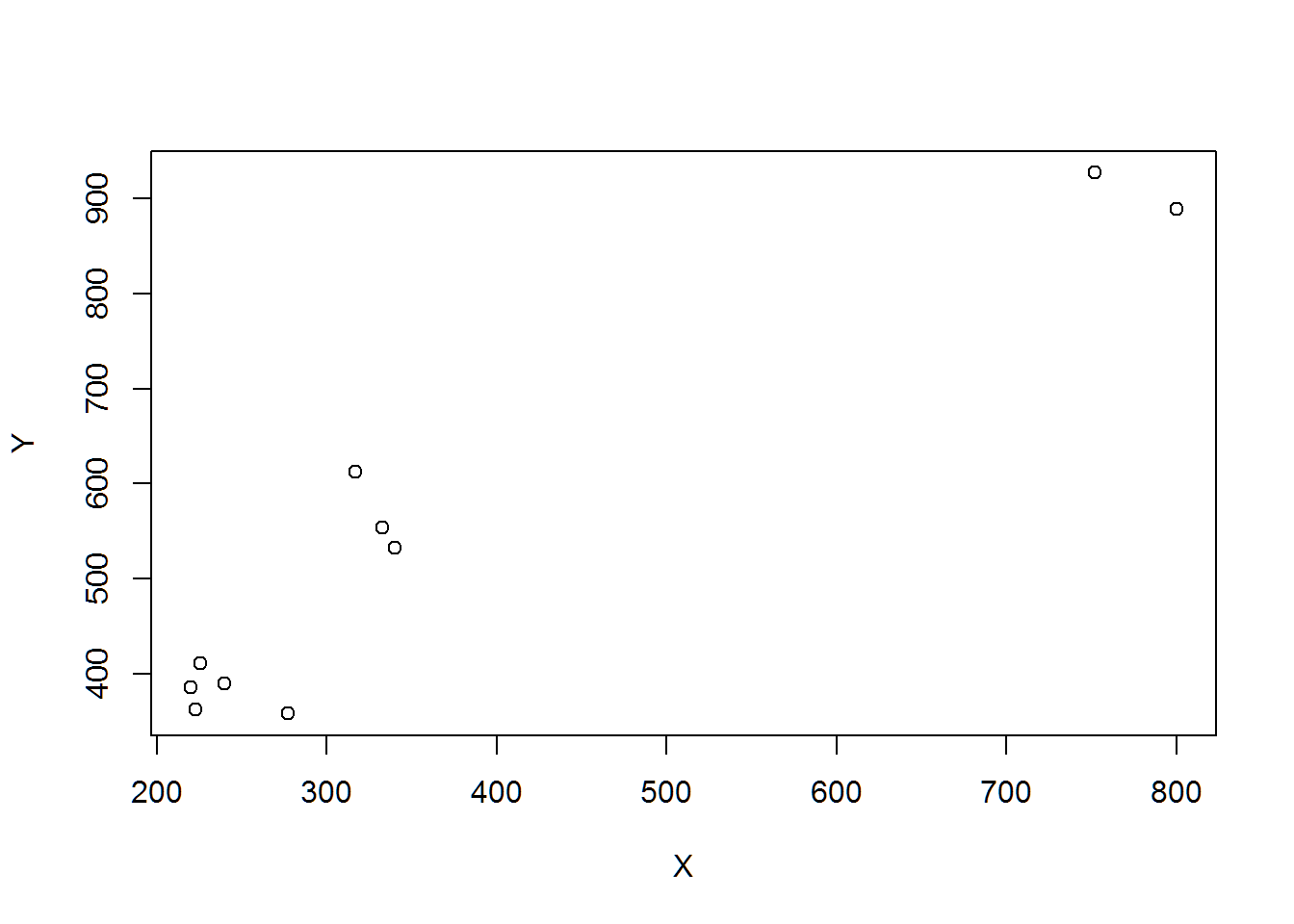
10 Conductivity
Cond = read.table(file.path(data.dir,"ToxAssesData.txt"),header=T)
# Akritas
with(Cond,{
  plot(X,Y)
})
# Hathaway
qplot(data=Cond,x=X,y=Y,size=I(2))+theme_bw()+labs(x="Surface Water Conductivity",y="Bank of River Conductivity")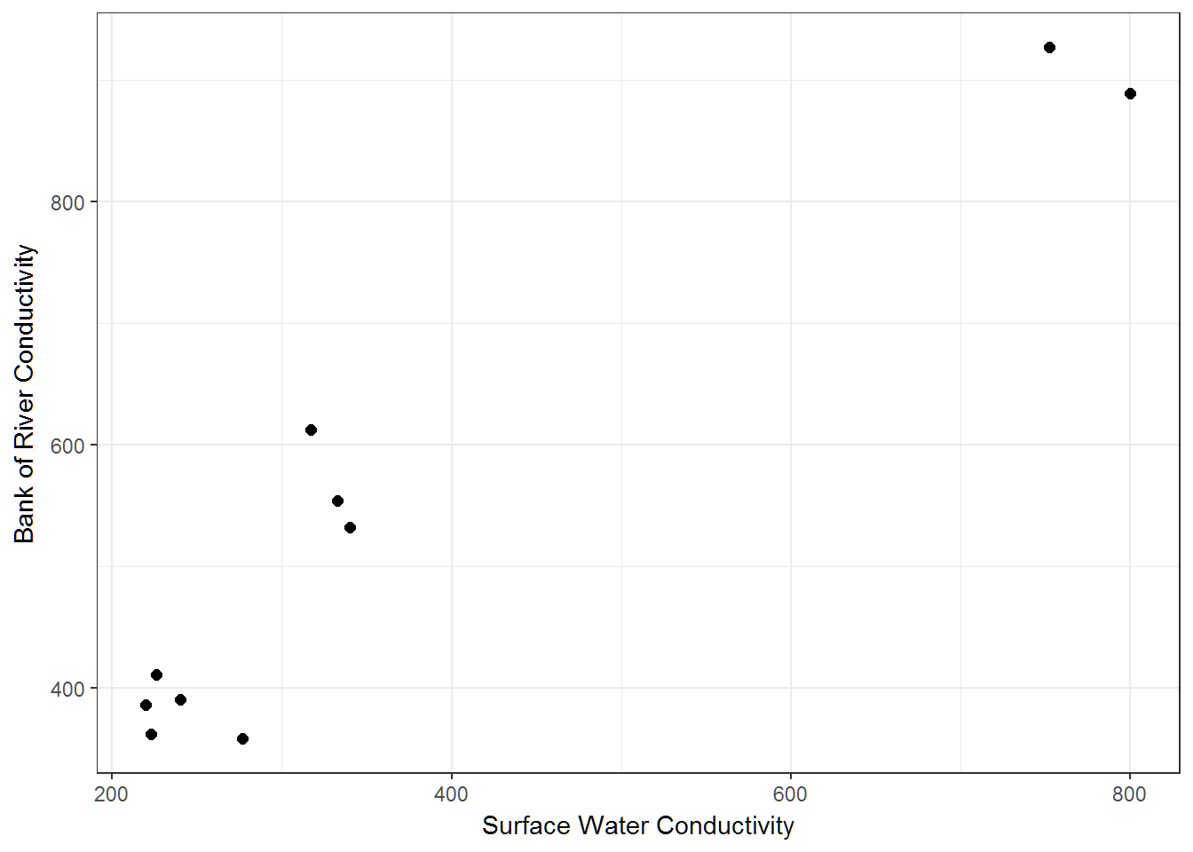
# Does there appear to be a relationship?  Yes.
# Is it positive or negative?
# Could there be a third variable accounting for the positive relationship?
13 Air Quality
### the object airquality is in R by default
# Akritas
pairs(airquality[1:5])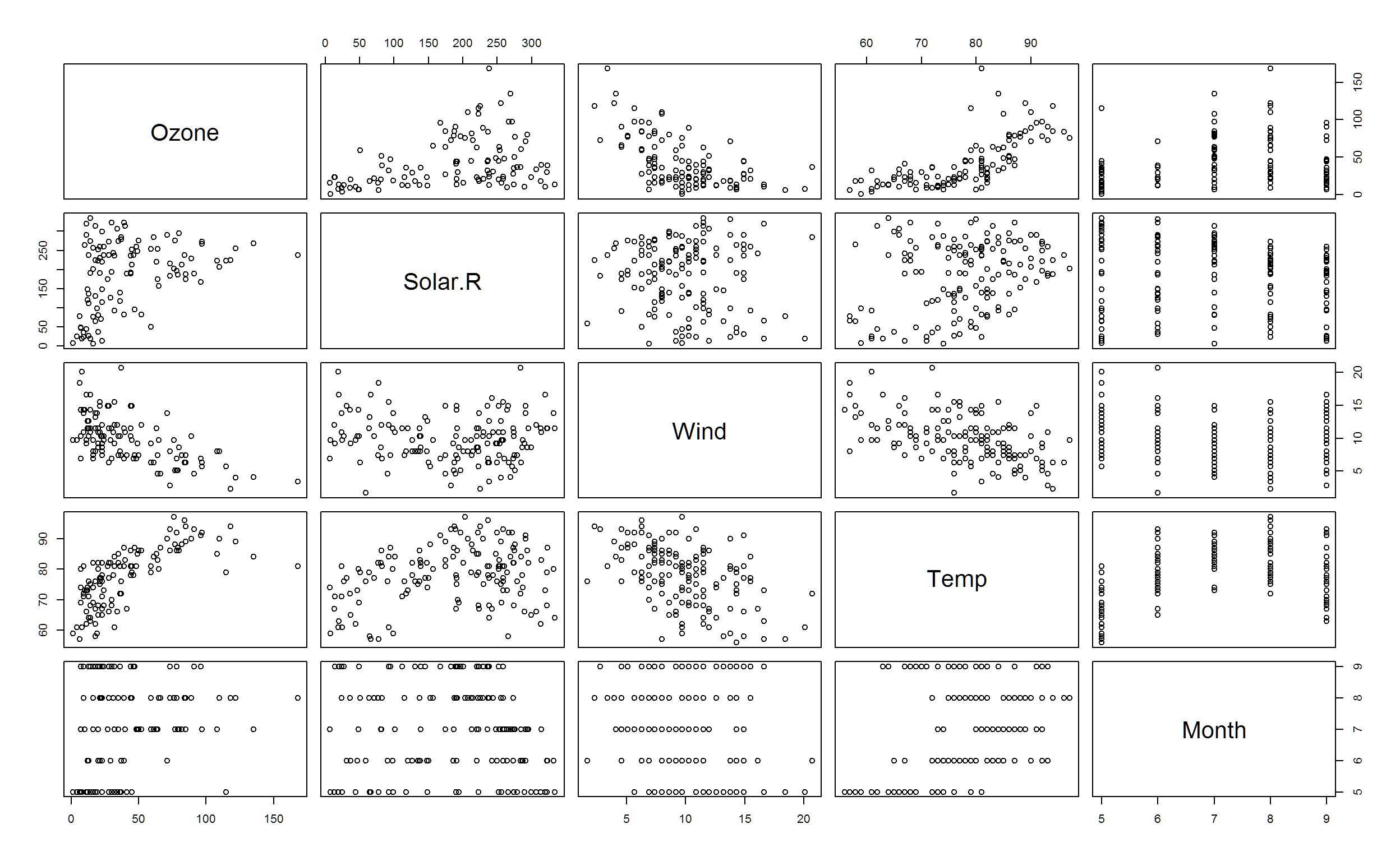
# Hathaway
library(GGally)
ggpairs(airquality,columns=1:5)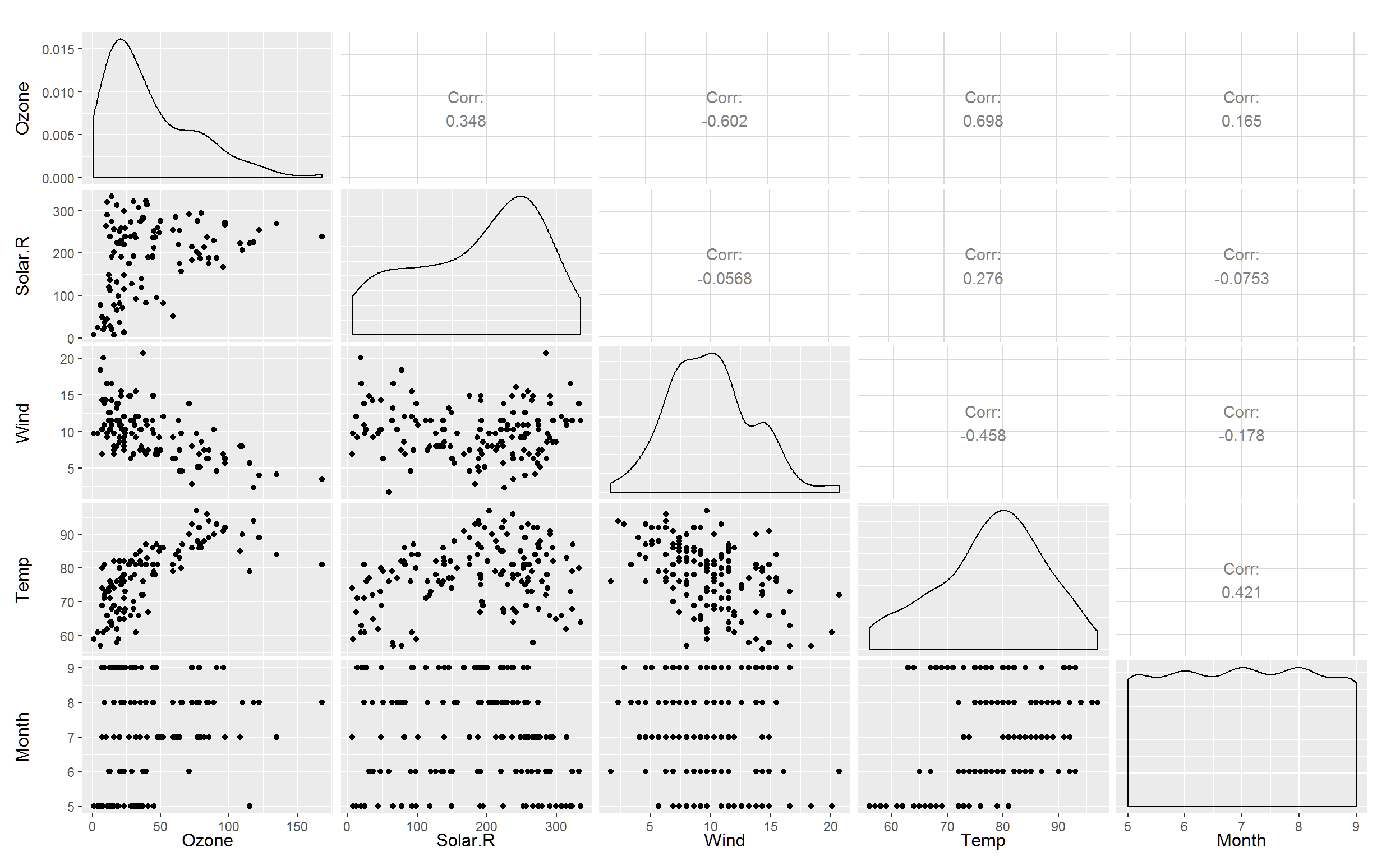
# If we set months as a categorical factor then
# air_tweak = airquality
# air_tweak$Month = factor(air_tweak$Month,levels=1:12)
#ggpairs(air_tweak,columns=1:5)
Extra Stuff you can ignore
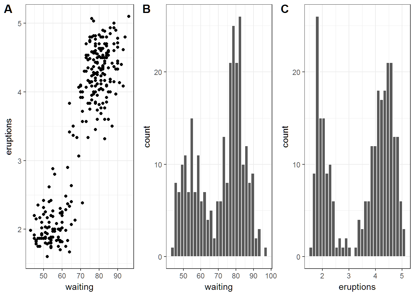
Old Faithfull
library(ggplot2)
library(cowplot)
## Warning: package 'cowplot' was built under R version 3.3.1## Warning: `legend.margin` must be specified using `margin()`. For the old
## behavior use legend.spacing##
## Attaching package: 'cowplot'## The following object is masked from 'package:ggplot2':
##
## ggsave#head(faithful)
p = ggplot(data=faithful)+theme_bw()
ps = p+geom_point(aes(x=waiting,y=eruptions))
phw = p+geom_histogram(aes(x=waiting),colour="white")
phe = p+ geom_histogram(aes(x=eruptions),colour="white")
plot_grid(ps,phw,phe,labels=c("A","B","C"),nrow=1)## `stat_bin()` using `bins = 30`. Pick better value with `binwidth`.## `stat_bin()` using `bins = 30`. Pick better value with `binwidth`.## Warning: `panel.margin` is deprecated. Please use `panel.spacing` property
## instead